
Chapter 4 - Models for Population Data
In this chapter, models for data from (animal or human) populations will be discussed. These models describe observations from a number of individuals sampled from the population. The distinguishing feature of the data to which such models apply is that there is more than one observation from some (usually most) individuals. A population model includes the structural model of Chapter 3, but also a new model, which shall be called the parameter model, for each individual’s kinetic parameters. The parameter model can have both fixed and random effects. A population model also includes the error model of Chapter 3.
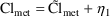
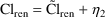
Individuals differ, and the types, degrees and causes of these differences are often what we want to learn. NONMEM was designed to help us learn these things. These individual differences can be due to fixed and/or random effects, but they all manifest themselves by affecting the value of an individual’s parameters,
. That is, first, each individual is regarded as
having his own particular value of
 . If the data come from
 individuals, then we may rewrite the (not completely)
general mixed effects model, (3.4) for
individuals, then we may rewrite the (not completely)
general mixed effects model, (3.4) for
 , the
, the
 observation from the
 individual, as

Eq (4.1) is now (part of)
a population model because it explicitly recognizes, through
the subscript,
 , that the data come from distinct individuals. Note too
that we have written
, that the data come from distinct individuals. Note too
that we have written
 , rather than
 . According to NONMEM conventions, when modeling data from a
population, the random effects in the residual errors
are denoted by
. According to NONMEM conventions, when modeling data from a
population, the random effects in the residual errors
are denoted by
 , their individual variances by
 , and the collection of the variances by the matrix
 , denoted SIGMA in NONMEM input and output. We also adopt
the same convention here as we did for
, denoted SIGMA in NONMEM input and output. We also adopt
the same convention here as we did for
 : the
: the
 diagonal element of
 is interchangeably denoted
 or
or
 .
.
When dealing with
population data, the symbol
 is reserved for random effects influencing the vectors
 , as is now explained. We can write a general model (but not
yet as general a model as we will present later) for
, as is now explained. We can write a general model (but not
yet as general a model as we will present later) for
 :
:

It is called the
parameter model. Here,
 is a structural (though non-kinetic) type model (of which
examples will be given shortly), which is a function of
fixed effects,
is a structural (though non-kinetic) type model (of which
examples will be given shortly), which is a function of
fixed effects,
 , and fixed effects parameters,
 . Note that since, in general,
 is a vector,
 must be a vector-valued function, and for the same reason,
 is usually a vector. This will be discussed further later.
All fixed effects, whether they are part of the kinetic
structural model, or are part of the parameter model, are
input to NONMEM in a uniform way. For the purposes of this
discussion, the symbol
is usually a vector. This will be discussed further later.
All fixed effects, whether they are part of the kinetic
structural model, or are part of the parameter model, are
input to NONMEM in a uniform way. For the purposes of this
discussion, the symbol
 is used for the particular fixed effects in
 , such as the individual’s height, weight, and so
forth (this will be discussed further in a moment). Even
though most often
, such as the individual’s height, weight, and so
forth (this will be discussed further in a moment). Even
though most often
 is regarded as time invariant, as is done in most of the
discussion in this document, fixed effects can change with
time, and thus kinetic parameters within
is regarded as time invariant, as is done in most of the
discussion in this document, fixed effects can change with
time, and thus kinetic parameters within
 can change with time. This will be discussed further in
Section 3.4.2.
can change with time. This will be discussed further in
Section 3.4.2.
The symbol in (4.2) for
the fixed effects parameter vector is
 , not
, not
 . As mentioned in Chapter 3, we reserve the symbol
 , in this document, for an individual’s fixed effect
parameters and use the symbol
, in this document, for an individual’s fixed effect
parameters and use the symbol
 for a vector of population (fixed effects and
possibly random effects) parameters.
for a vector of population (fixed effects and
possibly random effects) parameters.
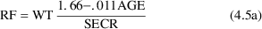
Recall the phenobarbital example of Chapter 2. For the second run, the input contained the line of code
TVCL = THETA(1) + THETA(3)*WT
Translated into the symbols we are using here, this is

In (4.3),
 and
and
 are the first and third elements of the parameter vector
 , and
, and
 is an element of
 (recall that this value of weight appears as a data item).
The tilde over
(recall that this value of weight appears as a data item).
The tilde over
 is meant to distinguish this typical population value of
clearance from the
is meant to distinguish this typical population value of
clearance from the
 individual’s actual value of clearance. According to
this model,
individual’s actual value of clearance. According to
this model,
 will be the same for any two individuals both of whom have
the same value of weight. Equation (4.3) defines an element
(the one associated with clearance) of the vector-valued
function
will be the same for any two individuals both of whom have
the same value of weight. Equation (4.3) defines an element
(the one associated with clearance) of the vector-valued
function
 . Note that in (4.3), we use the subscript
 to stress that this equation applies to the
 individual, but there is no confusion when, as in the
NM-TRAN input, and in the following, the subscript is
omitted. It should always be understood that all variables
and data items used in the parameter model definition refer
to the same individual. Many different models are possible
to describe the dependence of individual parameters on fixed
effects. However, certain model forms are simple, easy to
use, and cover most cases. An assortment of these will be
discussed briefly next.
individual, but there is no confusion when, as in the
NM-TRAN input, and in the following, the subscript is
omitted. It should always be understood that all variables
and data items used in the parameter model definition refer
to the same individual. Many different models are possible
to describe the dependence of individual parameters on fixed
effects. However, certain model forms are simple, easy to
use, and cover most cases. An assortment of these will be
discussed briefly next.
The simplest form that
 can take, and the most common, is one that is linear in
 . An example is (4.3): all elements of
 appear as linear coefficients of terms involving data items.
The data items themselves can appear nonlinearly, without
affecting the linearity with respect to
appear as linear coefficients of terms involving data items.
The data items themselves can appear nonlinearly, without
affecting the linearity with respect to
 . For example, if clearance is the sum of renal and
non-renal components, and renal clearance is believed to be
proportional to renal function as described according to a
standard formula involving the elements of
. For example, if clearance is the sum of renal and
non-renal components, and renal clearance is believed to be
proportional to renal function as described according to a
standard formula involving the elements of
 : age (
 ), serum creatinine (
 ), and weight (
 ), then one might write


Clearly,
 is a nonlinear function of
 , for example, and so, therefore, is
 , but
, but
 is linear in
 , and (4.4 - 4.6) is still considered a linear model. (Do
not worry about the non-consecutive numbering of the
elements of
, and (4.4 - 4.6) is still considered a linear model. (Do
not worry about the non-consecutive numbering of the
elements of
 ; a model for
 is being developed (an alternative to 4.3), and the missing
elements
is being developed (an alternative to 4.3), and the missing
elements
 and
and
 will appear presently.)
Multiplicative models are linear models, but on a logarithmic scale. For example, if patients covering a very wide range of weights are studied, metabolic clearance might vary with weight, but not linearly, and a substitute for (4.4) might be

Note that the logarithm
of
 (
(
 ) is linear in
 , but
, but
 itself is not. Of course, (4.4.1) can also be
written
itself is not. Of course, (4.4.1) can also be
written

Models (4.4.1) and
(4.4.2) are equivalent so far as
 is concerned, but
 of (4.4.2) corresponds to
 of (4.4.1).
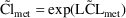
A useful model for
processes reaching a maximum is a hyperbolic model. For
example, if a second drug, (whose steady-state plasma
concentration,
 is known and available in the data set), is present in some
individuals and it is believed that this second drug is an
inhibitor of the metabolism of the study drug, one might
wish to use
is known and available in the data set), is present in some
individuals and it is believed that this second drug is an
inhibitor of the metabolism of the study drug, one might
wish to use
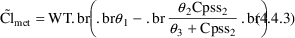
This model is shown in
figure 4.1. The inhibition is expressed by the ratio
occurring within the brackets and is a concave hyperbola,
asymptoting to a maximum value equal to
 . It is identical in form to the familiar Michaelis-Menten
model.
. It is identical in form to the familiar Michaelis-Menten
model.
Figure 4.1. A
hyperbolic model for metabolic clearance of drug on the
ordinate, as inhibited by another drug at steady-state
concentration
 on the abscissa.
Indicator variables were
discussed in Chapter 3 in connection with the error model.
They can be quite useful when modelling individual
parameters. They are usually used in a linear model. For
example, if the clinical condition, heart failure, is noted
as "present" or "absent", one can define
an indicator variable,
 which equals 0 if heart failure is absent, and 1 if it is
present. If metabolic clearance is thought to be affected by
heart failure, one might choose
which equals 0 if heart failure is absent, and 1 if it is
present. If metabolic clearance is thought to be affected by
heart failure, one might choose

Here, the
non-heart-failure cases will have
 , while the heart-failure cases will have
 †.
†.
----------
† Heart
failure is expected to decrease metabolic clearance. If it
does, using a minus sign in (4.4.4) allows the more pleasing
result that
 will be estimated as positive. The model is identical to one
with a positive sign, but then
will be estimated as positive. The model is identical to one
with a positive sign, but then
 would probably be negative. If
 were constrained to be non-negative, then the sign chosen in
the model statement would, of course, be important.
were constrained to be non-negative, then the sign chosen in
the model statement would, of course, be important.
----------
Given the basic building
blocks of linear, multiplicative and saturation models,
these can be combined in the usual algebraic ways (usually
by addition) to make more complex models. For example, one
could use (4.4.3), (4.5), and (4.6) as a model for
 . A non-additive example arises if plasma and urine
concentrations are both observed and (kinetic) model (3.6)
is to be used for the latter. The parameter
. A non-additive example arises if plasma and urine
concentrations are both observed and (kinetic) model (3.6)
is to be used for the latter. The parameter
 , the fraction of drug excreted unchanged into the urine
might be modeled as
, the fraction of drug excreted unchanged into the urine
might be modeled as
where
 is given by (4.5) and
 by (4.6) (using any of the (4.4) variants).
As mentioned in Section
2, although most of the time the data items affecting an
individual’s
 do not change over the course of his data, they occasionally
do, and PREDPP can handle this. For example, if an
individual had heart failure for part of his observation
period, but not the rest,
do not change over the course of his data, they occasionally
do, and PREDPP can handle this. For example, if an
individual had heart failure for part of his observation
period, but not the rest,
 , according to (4.4.4) should change. Or, if acute renal
failure occurred during a patient’s observation
period,
, according to (4.4.4) should change. Or, if acute renal
failure occurred during a patient’s observation
period,
 would change, according to model (4.5).
PREDPP implements its
kinetic model recursively: given the state of the system at
time
 (by state we mean the amounts of drug in all the
compartments), it updates (i.e. advances) the state to that
at time
(by state we mean the amounts of drug in all the
compartments), it updates (i.e. advances) the state to that
at time
 , using the value of
 (and in general, the value of
 ) at time
 to compute a value of
 holding between times
 and
and
 . The value of
 used to compute this
 is that value found on the data record with time
 . So, in order to have
 change appropriately as
 does, one places a value of
 which is typical for the time period
 to
to
 on the data record associated with the time point
 . This will not always be easy since the relevant element(s)
of
. This will not always be easy since the relevant element(s)
of
 may not be measured at, for example, the midpoint of the
time interval (the value at the
may not be measured at, for example, the midpoint of the
time interval (the value at the
 of the time interval is a good choice for the
 value for the interval). If not, one will have to use some
interpolation method to arrive at the typical value. The
important point is that the values of the independent
variables at time
value for the interval). If not, one will have to use some
interpolation method to arrive at the typical value. The
important point is that the values of the independent
variables at time
 determine the values of the individual’s parameters
applying to the entire period
determine the values of the individual’s parameters
applying to the entire period
 to
to
 .
.
The kinetic models (i.e.,
the models for responses such as drug concentrations) used
when performing a population analysis do not differ at all
from those used for an individual analysis. One still needs
a model for the relationship of
 to
to
 and
and
 , and this relationship does not depend on whether
 changes from individual to individual or with time within an
individual.
changes from individual to individual or with time within an
individual.
Under NONMEM conventions,
there are two levels of random effects, and
 and
and
 are the symbols used for the vectors of first and second
level random effects, respectively. With data from a single
individual, only first-level random effects are needed.
However, with data from a population of individuals, both
first- and second-level random effects are needed.
First-level effects are needed in the parameter model to
help model unexplainable interindividual differences in
are the symbols used for the vectors of first and second
level random effects, respectively. With data from a single
individual, only first-level random effects are needed.
However, with data from a population of individuals, both
first- and second-level random effects are needed.
First-level effects are needed in the parameter model to
help model unexplainable interindividual differences in
 , and second-level effects are needed in the
(intraindividual) error model. For example, in (4.2) there
is an element of
, and second-level effects are needed in the
(intraindividual) error model. For example, in (4.2) there
is an element of
 ,
,
 , that is the difference between the individual value
 (an element of
 ) and
) and
 , the typical value of
 . This is a first-level random effect. In (4.1)
 is the error between
 and
and
 . This is a second-level random effect.
The difference between
 and
and
 is called an interindividual error. It arises from a
few sources: the function
is called an interindividual error. It arises from a
few sources: the function
 may be only approximate, and/or
 may be measured with error. It is regarded as a random
quantity, and it may be modeled in terms of
may be measured with error. It is regarded as a random
quantity, and it may be modeled in terms of
 variables. As usual, each of these variables is assumed to
have mean 0 and a variance denoted by
variables. As usual, each of these variables is assumed to
have mean 0 and a variance denoted by
 which may be estimated. This variance describes biological
population variability.
which may be estimated. This variance describes biological
population variability.
The difference between
 and
and
 is called an intraindividual error. It has been
discussed at some length in Chapter 3. Although in that
discussion about individual data, this difference was
modeled in terms of
is called an intraindividual error. It has been
discussed at some length in Chapter 3. Although in that
discussion about individual data, this difference was
modeled in terms of
 variables, in this discussion about population data, it is
modeled in terms of
variables, in this discussion about population data, it is
modeled in terms of
 variables. Each
 variable is assumed to have mean 0 and a variance denoted by
 which also may be estimated.
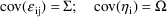
Each pair of elements in
 has a covariance, and NONMEM can also estimate this,
although often we choose to assume that the covariance is
zero (we made this same assumption for the different
elements of
has a covariance, and NONMEM can also estimate this,
although often we choose to assume that the covariance is
zero (we made this same assumption for the different
elements of
 in Chapter 3, Section 3.5.1).
A covariance between two elements of
 ,
,
 and
and
 , say, is a measure of statistical association between these
two random variables. Their covariance is related to their
correlation,
, say, is a measure of statistical association between these
two random variables. Their covariance is related to their
correlation,
 (
(
 ) by
) by

(Note that now that we
are suppressing the subscript
 on
on
 , we may, without confusion, use the subscript position to
designate elements of
, we may, without confusion, use the subscript position to
designate elements of
 .)
.)
The variances and
covariances among the elements of
 are laid out in a covariance matrix, called
 , and labeled OMEGA in NONMEM input and output. This matrix
was defined in Chapter 3, Section 3.8, but some additional
comment here may be helpful. If
, and labeled OMEGA in NONMEM input and output. This matrix
was defined in Chapter 3, Section 3.8, but some additional
comment here may be helpful. If
 has, for example, 3 elements,
 has the following form:
Here, as previously,
 is another way of writing the variance
 , and
, and
 (
(
 ) is the covariance between
 and
and
 .
.
The elements
 ,
,
 ,
,
 are called the diagonal elements of the matrix. If
the nondiagonal elements (the covariances) are all zero,
i.e. the correlation among all pairs of
are called the diagonal elements of the matrix. If
the nondiagonal elements (the covariances) are all zero,
i.e. the correlation among all pairs of
 elements is zero, the matrix is called a diagonal matrix.
The lower triangular elements of the matrix are the
elements
elements is zero, the matrix is called a diagonal matrix.
The lower triangular elements of the matrix are the
elements
To specify the matrix only its lower triangular elements
need be given (and these are all NONMEM does give), since
from (4.8) it is clear that for all
 ,
,
 .
.
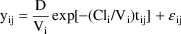
Frequently, the model for an interindividual error is the simple additive one (as in (4.2)), such as

A feature of (4.9) is that the
resulting units for
 depend on the units of the parameter (
 in this case). For example, this model was used in the
theophylline problem of Chapter 2 (Figure 2.6). The final
estimate of
in this case). For example, this model was used in the
theophylline problem of Chapter 2 (Figure 2.6). The final
estimate of
 is .286 (Figure 2.8). Assuming that the units of V are
liters, we interpret this to mean that the standard
deviation of V between individuals is .53 Liters ( .53 =
is .286 (Figure 2.8). Assuming that the units of V are
liters, we interpret this to mean that the standard
deviation of V between individuals is .53 Liters ( .53 =
 ).
).
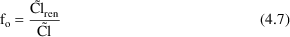
Perhaps even more often, a multiplicative model equivalent to the Constant Coefficient of Variation (CCV) error model (3.5) is used, such as

This model is also referred to
as the proportional error model.
A feature of (4.10) is that the resulting units for
 are independent of the units of the parameter (
 in this case). When this model is used in the theophylline
problem instead of the additive model, so that Figure 2.6
contains the code V=TVVD*(1+ETA(2)) instead of
V=TVVD+ETA(2), then NONMEM estimates
in this case). When this model is used in the theophylline
problem instead of the additive model, so that Figure 2.6
contains the code V=TVVD*(1+ETA(2)) instead of
V=TVVD+ETA(2), then NONMEM estimates
 to be .146. We interpret this to mean that the coefficient
of variation of V in the population is 38% (.38 =
to be .146. We interpret this to mean that the coefficient
of variation of V in the population is 38% (.38 =
 ).
).
The exponential model is

During simulation, (Chapter 12, Section 4.8), the exponential and proportional models give different results. During estimation by the first-order method, the exponential model and proportional models give identical results, i.e., NONMEM cannot distinguish between them. During estimation by a conditional estimation method, the exponential and proportional models for inter-individual variability give different results. The exponential model is preferred for conditional estimation methods. (See NONMEM User’s Guide Part VII, Conditional Estimation Methods.)
Occasionally, a model for an
individual’s pharmacokinetic parameter might involve
scaling an
 , as in (3.6), or two or more
 ’s as in (3.10). For example, a study might involve
patients in the intensive care unit (ICU) and others on
non-acute care units. It might be reasonable to suppose that
some aspects of the kinetics of ICU patients (e.g.,
metabolic clearance of drug) are more variable, due to
unmeasured factors (e.g., hepatic function) that vary
greatly among acutely ill patients. Even though the
variation is, in reality, due to a potentially measurable
fixed effect (hepatic function), if information on this
fixed effect is not available, differences caused by it must
be assigned to random factors (
’s as in (3.10). For example, a study might involve
patients in the intensive care unit (ICU) and others on
non-acute care units. It might be reasonable to suppose that
some aspects of the kinetics of ICU patients (e.g.,
metabolic clearance of drug) are more variable, due to
unmeasured factors (e.g., hepatic function) that vary
greatly among acutely ill patients. Even though the
variation is, in reality, due to a potentially measurable
fixed effect (hepatic function), if information on this
fixed effect is not available, differences caused by it must
be assigned to random factors (
 ). In this case, one might wish to use an indicator
variable,
). In this case, one might wish to use an indicator
variable,
 (which equals 1 if the patient is in the ICU, and 0,
otherwise), and a model such as
(which equals 1 if the patient is in the ICU, and 0,
otherwise), and a model such as

In addition to model (4.11) we might have, for example,


Models (4.11) and (4.12)
together, along with suitable models for
 and
and
 , form a complete model for an individual’s
 parameter, and involve 3
 ’s.
’s.
As we have just seen in (4.10)
and in (4.11)-(4.12), an element of
 need not act in a simple additive way and may act solely on
an intermediate variable (e.g.
need not act in a simple additive way and may act solely on
an intermediate variable (e.g.
 ). Indeed, there may be more or fewer elements in
 than in
 , the elements in
 may act in nonlinear ways to influence
 , and one element of
 may influence more than a single element of
 . We now give a more general form for the parameter model
than (4.2) and then an example illustrating it.
. We now give a more general form for the parameter model
than (4.2) and then an example illustrating it.
The general form of the parameter model is

Here,
 is a very general function of fixed effects,
 , fixed effects parameters,
 , and a vector of
 ’s,
’s,
 . The dimensions of the vectors
 and
and
 need not be the same. An individual’s kinetic
parameter may change with time. As explained in Section 1.6,
with NONMEM-PREDPP changes can occur only at discrete time
points. Therefore, the parameter actually can be regarded as
being a number of parameters, each one applying to a
different time period. The parameter
need not be the same. An individual’s kinetic
parameter may change with time. As explained in Section 1.6,
with NONMEM-PREDPP changes can occur only at discrete time
points. Therefore, the parameter actually can be regarded as
being a number of parameters, each one applying to a
different time period. The parameter
 in (4.13), being a vector of all the kinetic parameters for
the
in (4.13), being a vector of all the kinetic parameters for
the
 individual, can be regarded as encompassing these
time-interval-specific parameters.
individual, can be regarded as encompassing these
time-interval-specific parameters.
An example utilizing this generality is provided by a model for observations of both plasma and urine drug concentrations, similar to the one presented previously. Ignoring the details of the structural part of the model, consider the following model


In this model,
 ; the parameters
 and
and
 are regarded as intermediate parameters. We have
 , where both
 and
and
 influence both
 (linearly) and
 (nonlinearly).
Model (4.1) can be generalized
by incorporating a model like those given in Chapter 3 for
the residual errors, i.e. for the differences between the
 and
and
 , rather than using just the simple Additive model. A
particular instance of such a model may have several types
of
, rather than using just the simple Additive model. A
particular instance of such a model may have several types
of
 ’s, and as mentioned in Section 2, the variances of
these
’s, and as mentioned in Section 2, the variances of
these
 ’s are denoted by
 ’s. With a population model these variances could
change from individual to individual. With NONMEM, they are
considered as constants over individuals. The
’s. With a population model these variances could
change from individual to individual. With NONMEM, they are
considered as constants over individuals. The
 ’s can co-vary. A covariance matrix
 , like the
 matrix given in Section 4.1, gives the variances and
covariances of the
matrix given in Section 4.1, gives the variances and
covariances of the
 ’s, as already discussed at the end of Chapter 3. This
does not preclude the magnitudes of the errors from being
affected by fixed effects. A model such as (3.8) can still
be used. This is shown explicitly by the general model given
in the next section.
’s, as already discussed at the end of Chapter 3. This
does not preclude the magnitudes of the errors from being
affected by fixed effects. A model such as (3.8) can still
be used. This is shown explicitly by the general model given
in the next section.
We have now presented all of the parts needed to fully define a population model. It may be useful to recap this information by stating the entire general model here:


 ,
,
 independent for

 ,
,
 independent for

 ,
,
 independent for all
 ,
,
where here,
 is a vector, along with
 ,
,
 ,
,
 and
and
 , and
, and
 and
and
 are square matrices with dimensions equal to those of
 and
and
 .
.
To try to represent the relationship between all the fixed and random effects of a population model graphically, consider figure 4.2. The model corresponding to this figure is


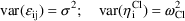
where the
 are all equal to a constant
 , i.e. there is no random interindividual variability in the
volume of distribution, so that for the sake of this
example,
, i.e. there is no random interindividual variability in the
volume of distribution, so that for the sake of this
example,
 is just a scalar.
Figure 4.2. Random and
fixed effects influence observation,
 , from the population point of view. Open circle, lower
left, is population parameter predicted clearance, closed
circle is true clearance for
, from the population point of view. Open circle, lower
left, is population parameter predicted clearance, closed
circle is true clearance for
 individual which differs from population prediction by
 , chosen randomly from a distribution (upper left) with mean
0 and SD
, chosen randomly from a distribution (upper left) with mean
0 and SD
 . Similarly, lower right, the observed
 at time
 (open square) differs by
 from the true value (closed circle) by an error
 , chosen independently from a distribution with mean 0 and
SD
, chosen independently from a distribution with mean 0 and
SD
 . The
. The
 corresponding to the population-based prediction is also
shown (upper curve, open circle).
corresponding to the population-based prediction is also
shown (upper curve, open circle).