NONMEM Users Guide Part V - Introductory Guide - Chapter 12

Chapter 12 - Brief Descriptions of Other Features

1. What This Chapter is About

This chapter briefly describes a variety of features of PREDPP and NONMEM that are somewhat advanced for this text but are of interest to most users of NONMEM. References are given to other documents where additional information can be found. Section 2 is concerned with PREDPP, Section 3 is concerned with user-written PREDs, and Section 4 describes general NONMEM features. Section 5 contains an example that includes several of the advanced features. Descriptions of NM-TRAN control records in Section 4 have been augmented with sections headed "More about ...". These contain additional details, plus new options for NONMEM 7.3. Section 6 is new for NONMEM 7.3. It contains a supplemental list of features through NONMEM 7.4, including features from previous releases that are not otherwise discussed in this guide.

Note that wherever $PK, $ERROR, $DES, $AES, $MODEL, $MIX, $INFN, $TOL and $PRED statements are referred to below, user-written subroutines PK, ERROR, DES, AES, MODEL, MIX, INFN, TOL and PRED can be used instead.

2. Advanced Features of PREDPP

2.1. Pharmacodynamic Modeling Using the $ERROR Record

$ERROR statements may modify the value of F, the scaled drug concentration. They may also introduce new and variables. This allows pharmacodynamic modeling to be performed using PREDPP. Such models occur when a study involves measurement of a drug effect, such as blood pressure. A proposed model might relate the predicted effect to a pharmacokinetic quantity such as plasma level. PREDPP can be used to model as is usual, and the predicted effect can be computed in the $ERROR statements.

For example, suppose that a modified version of the phenobarbital data of Chapter 2 includes observations of some drug effect (in this case, perhaps a measure of the degree of sedation) but none of the concentration observations. The dose event records are the same as those of the earlier example. Suppose that the drug concentrations from each individual have been used to estimate that individual’s K and V parameters, and that these estimates are now included on every event record for the individual. Finally, suppose that the proposed structural model for the effect, E, is an "E-max" model:

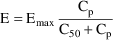
where here is understood to mean the prediction of an individual’s drug concentration in the plasma, and and are PD (pharmacodynamic parameters) modeled as

To fit this data we can use the control statements of figure 12.1. To obtain initial parameter estimates, let us assume that the following is observable in the data. The average value of all effect measurements is about 50. Across individuals, the average value of the largest effect measurement within each individual’s data is about 100, and the average value of the individual’s observed concentration at about half this largest measurement is about 20. (This is seen when concentration measurements and effect measurements are examined together.) Let us also assume 20% random interindividual variability in and and 4% intraindividual variability in the observation. From this we obtain initial estimates of 100 and 20 for and , for , for , and for .

This example is examined again in in Section 3.2, which shows the use of $PRED statements, and in Section 5, which shows how observed concentrations and effects can be fit simultaneously.

References: Users Guide VI (PREDPP) IV.B.2

$PROBLEM PHARMACODYNAMIC MODEL USING $ERROR STATEMENTS
$INPUT   ID TIME AMT INDK INDV DV
$DATA    EFFDATA
$SUBROUTINE ADVAN1
$PK
   K=INDK
   V=INDV
   S1=V
$ERROR
 EMAX=THETA(1)+ETA(1)
 C50=THETA(2)+ETA(2)
 E=EMAX*F/(C50+F)
 Y=E+ERR(1)


$THETA   100  20
$OMEGA   400  16
$SIGMA   4
$ESTIMATION

Figure 12.1. The input to NONMEM-PREDPP for analysis of effect observations.

2.2. Other Pharmacokinetic Models: ADVAN5-9,ADVAN13-18

Appendix 1 lists ADVAN routines for the most commonly-used pharmacokinetic models. Other ADVAN routines are:
ADVAN5 (General Linear)
ADVAN6 (General Nonlinear)
ADVAN7 (General Linear with Real Eigenvalues)
ADVAN8 (General Nonlinear Kinetics with Stiff Equations)
ADVAN9 (General Nonlinear Kinetics with Equilibrium Compartments)
ADVAN13 (General Nonlinear Kinetics With Stiff/Nonstiff Equations using LSODA)(nm71)
ADVAN14 (General Nonlinear Kinetics With Stiff/Nonstiff Equations using CVODES)(nm74)
ADVAN15 (General Nonlinear Kinetics with Equilibrium Compartments using IDAS)(nm74)
ADVAN16 (General Nonlinear Kinetics with Stiff/Nonstiff and Delay Equations using RADAR5 (nm75)
ADVAN17 (General Nonlinear Kinetics with Equilibrium Compartments using RADAR5)(nm75)
ADVAN18 (General Nonlinear Kinetics with Nonstiff and Delay Equations using DDE_SOLVER (nm75)

With the general methods the user defines a model of up to 999 compartments using special options of the $MODEL record. For a linear model (ADVAN5 and ADVAN7), it is sufficient to specify (directed) compartmental connections and to compute their rate constant parameters with $PK statements. ADVAN 5 and 7 make use of numerical approximations to the matrix exponential. For a nonlinear model (ADVAN6, ADVAN8, ADVAN9, ADVAN13, ADVAN14, ADVAN15, ADVAN16, ADVAN17, ADVAN18), differential equations must be supplied to govern the kinetics, via $DES statements. It is possible to specify initial conditions for the differential equations using the I_SS (Initial Steady State) feature; Reserved variable ISSMOD may be used.

For ADVAN9, ADVAN15 and ADVAN17, algebraic equations may also be supplied via $AES statements.

The use of the term ’nonlinear’ with ADVAN 6, 8, 9, 13, 14, 15, 16, 17, 18, only indicates that a system of any type of first-order differential equations is allowed; such equations could be linear or non-linear.

In all cases, the basic features of PREDPP described in Chapter 7 are still available, such as the ability to introduce doses of any kind to any compartment of the model. It should be noted that the general ADVAN routines are relatively slow. For example, when a general method is used for a model identical to that of an analytic method (ADVAN1 through ADVAN4 or ADVAN10 through ADVAN12) the run time increases, usually by an order of magnitude.

Some ADVAN and SS routines must be told the number of accurate digits that are required in the computation of drug amounts, i.e., the relative tolerance. They may also be told the absolute tolerance. With some ADVAN and SS, the tolerances may be specified for each compartment. They may be specified by $SUBROUTINES record options TOL, ATOL, SSTOL, SSATOL; by the corresponding options of the $TOL record; or by user-written subroutine TOL (which may also specify tolerances by NONMEM Step). Option TOL (relative tolerance) may also be specified on the $COVARIANCE record. Option ATOL (absolute tolerance) may also be specified on $ESTIMATION and $COVARIANCE records.

See Guide NONMEM 7, "Controlling the Accuracy of the Gradient Evaluation and Individual Objective Function Evaluation"

With ADVAN9, ADVAN13, ADVAN14, and ADVAN15, reserved variable MXSTEP may be used to set the number of integration steps.

With $AES, $AESINIT statements are also required. If there is no TIME data item, $AESINIT may specify a calling protocol for the AES subroutine. (See 2.7 below for a discussion of calling protocols.)

Call ADVAN9 and ADVAN15 and AES with every event record (default)

Call ADVAN9 and ADVAN15 and AES once per individual record.

Equivalent calling protocol phrases are:

(EVERY EVENT)
(ONCE PER IR)

References: Users Guide VI (PREDPP) VI, VII
References: Users Guide IV (NM-TRAN) V.C.3, 4, 7-10

2.3. Zero-Order Bolus Doses

Instantaneous bolus doses, which have AMT>0 and RATE=0, are described in Chapter 6. Such doses appear instantaneously in the dose compartment. Zero-order bolus doses are doses that enter the dose compartment via a zero-order process (in the same manner as do infusions) except that the rate or duration of the process is computed with $PK statements. When the RATE data item has the value -1, then the $PK statements must include an assignment statement for an additional PK parameter, Rn (the "modeled rate for compartment n"), whose value gives the rate of entry of the drug during the interval of time between the last event record and the current one. There is a different such parameter for every compartment receiving a zero-order bolus dose. When the RATE data item has the value -2, then the $PK statements must include an assignment statement for an additional PK parameter, Dn (the "modeled duration for compartment n"), whose value at the time of the dose event gives the duration time of the dose. The rate and duration parameters can be modeled like any other PK parameters; in particular, the assignment statements can involve ’s which are to be estimated. These parameters can be used to model the drug release rate or dissolution time of a tablet or capsule.

Steady-state levels involving zero-order bolus doses can be computed.

Steady-state with constant infusion was described in Chapter 6. Steady-state infusions may also have modeled rates (i.e., the RATE data item may be -1).

References: Users Guide VI (PREDPP) III.F.3, F.4

2.4. The Additional Dose Data Item: ADDL

ADDL is a dose-related data item that is used to request that a given number of additional doses, just like the dose specified on the event record, be added to the system at a regular time interval, starting from the time on the event record. PREDPP itself adds these doses at the appropriate future times; no actual dose event record is generated by the Data Preprocessor or by PREDPP. A positive integer value in ADDL specifies how many additional doses (i.e., in addition to that already specified in the event record) are to be given, and the value in the II (interdose interval) data item (which is required) specifies the time interval between doses.

ADDL may be non-zero on a steady-state dose event record (except for steady-state infusions), in which case additional doses are given, maintaining the dosing regimen into the future. Non-steady-state kinetic formulas are used to advance the system between each additional dose. Reserved variables DOSTIM (the time of a lagged dose or additional dose to which the system is being advanced) and DOSREC (the dose record corresponding to the dose entering at DOSTIM) may be used.
See also Section 2.6 below.

References: Users Guide VI (PREDPP) V.K

2.5. Lagged doses: the ALAG Parameter

PREDPP permits an additional PK parameter called an absorption lag time. One such parameter can be defined for each compartment and applies to all doses to that compartment. It gives the amount of time that a dose is held as a "pending" dose. When the absorption lag time has expired, the dose is input into the system. In effect, the value of the absorption lag time parameter is added to the value of the TIME data item on the dose event record. With NM-TRAN, recognized names for absorption lag time parameters have the form ALAGn, where n is the compartment number. Reserved variables DOSTIM (the time of a lagged dose or additional dose to which the system is being advanced) and DOSREC (the dose record corresponding to the dose entering at DOSTIM) may be used.
See also Section 2.6 below.

See Guide VI, Chapter V, Note 3 for the effect of ALAGn with Steady-State doses.

References: Users Guide VI (PREDPP) III.F.6
References: Users Guide IV (NM-TRAN) V.C.5

2.6. Model Event Times: MTIME

Model event times MTIME(i) are additional PK parameters defined in the PK routine or $PK block. A model event time is not associated with any compartment, but, like an absorption lag time, defines a time to which the system is advanced. When the time is reached, indicator variables are set and a call to PK is made. At this call (and/or subsequent to this call) PK or DES or AES or ERROR can use the indicator variables to change some aspect of the system, e.g., a term in a differential equation, or the rate of an infusion. Reserved variables MNEXT, MPAST, MNOW, MTDIFF may be used.

MTIME does not apply to Steady-State doses. See Guide VI, Chapter V, Note 4.

2.7. Controlling Calls to PK and ERROR

In order to evaluate the $PK and $ERROR statements, PREDPP calls the PK and ERROR subroutines. By default, the subroutines are called with every event record. PREDPP may be instructed to limit calls to certain event records in order to save the computing time involved with unnecessary calls (e.g. when the PK parameters do not vary from event record to event record within an individual). It is also possible to cause the PK subroutine to be called at times which do not correspond to any actual event record.

Using NM-TRAN, calls to PK are controlled by the presence of one of the following pseudo-statements, at the start of the $PK block:

call with every event record, at additional and lagged dose times, and at modeled event times.

call with every event record (default).

call with the first event record of each individual record and with new values of TIME.

call once per individual record.

A calling protocol phrase may be used instead of a pseudo-statement. A calling protocol phrase may use upper- or lower-case characters. It must be enclosed in parentheses. NM-TRAN can understand minor variations in the wording. E.g., the word "CALL" and prepositions such as WITH can be omitted. Here are calling protocol phrases equivalent to the above four pseudo-statements, respectively.

(CALL WITH NON-EVENT TIMES)
(CALL WITH EVERY EVENT RECORD)
(CALL WITH FIRST EVENT RECORD AND NEW TIME)
(CALL ONCE PER INDIVIDUAL RECORD)

The choice CALLFL=-2 (CALL WITH NON-EVENT TIMES) is intended to be used when PK parameters Dn and/or Fn apply to additional or lagged doses and the model for these parameters depends on some time-varying concomitant variable such as type of drug preparation or patient weight. By default, the values of the PK parameters which apply to the dose are those values computed by PK with the first event record having a value of TIME greater than the time at which the dose actually enters the system (the additional or lagged dose time). However, if PREDPP is instructed to also call PK at the additional or lagged dose time, then the values of the PK parameters are those values computed at these special calls. At such calls, PK has available to it information from the initiating dose event record itself, and information from the two event records whose TIME values bracket the additional or lagged dose time. Along with CALLFL=-2 in the $PK block, the NM-TRAN $BIND record may be useful; see Users Guide IV.
Using NM-TRAN, calls to ERROR are controlled by the presence of one of the following pseudo-statements at the start of the $ERROR block:

A calling protocol phrase may be used instead of a pseudo-statement. As in the $PK block, the calling protocol phrase may use upper- or lower-case characters and must be enclosed in parentheses.
Here are calling protocol phrases equivalent to the above three pseudo-statements, respectively.

(CALL WITH EVERY EVENT RECORD)
(CALL WITH OBSERVATION EVENTS)
(CALL ONCE PER INDIVIDUAL RECORD)

NM-TRAN automatically instructs PREDPP to limit calls to ERROR to once per problem for the simple error models discussed in Chapter 8, Sections 3.1 and 3.2:
Y=F+ERR(1)
Y=F+F*ERR(1)
Y=F*(1+ERR(1))
Y=F*EXP(ERR(1))
During the Simulation Step, PREDPP ignores any limitation and calls the ERROR subroutine with every event record.
Even when calls to PK and/or ERROR are limited, the CALL input data item can be used to force additional calls for specific event records as needed.
References: Users Guide VI (PREDPP) III.B.2, III.H, IV.C, V.J
References: Users Guide IV (NM-TRAN) V.C.5, C.6

2.8. Output-Type Compartments

With all versions of PREDPP output-type compartments may be defined using the $MODEL record. Suppose there is a compartment named METABURI (for metabolite in urine). If it is to be an output-type compartment, it must defined as follows:
$MODEL COMP=(METABURI,NODOSE,INITIALOFF)
The compartment is initally off, may be turned on and off, and may not receive a dose. Just as with the default output compartment, CMT may be negative on an observation record, allowing the observation to be obtained, and then the compartment turned off, with a single record. There may be more than one such compartment, in addition to the default output compartment. An output-type compartment must be turned on with an other-type event record in order to start accumulating drug. An output-type is not computed by mass-balance, but must instead be computed explictly by the ADVAN routine, e.g., using a differential equation when a general non-linear model is used.
For an example, see Chapter 6, Section 9.

 ID  TIME EVID UVOL  DV   CMT  AMT
  1  9.50   0   75  .058   -3    0

With ADVAN2, compartment 3 is the default compartment for output, and the observation at TIME 9.50 may have CMT=-3. But suppose a general linear or non-linear model is used (ADVAN5,6,7,8,9,13) and there are more than 3 user-defined compartments.
If the $MODEL statement describes the 3d. compartment as simply
$MODEL COMP=NAME
then the default compartment attributes apply (initial on, off/on allowed, dose allowed) and the compartment is not an output-type compartment. PREDPP produces this error message for data record 3:
SPECIFIED COMPARTMENT MAY NOT BE TURNED OFF WITH AN OBSERVATION RECORD
There are two ways to avoid this error message. First, it is always possible (for any compartment that may be turned off, even the output compartment) to use two records instead of one, e.g., first the observation, then a record with EVID=2 that turns off the compartment:

  1  9.50   0   75  .058    3    0
  1  9.50   2    0   0     -3    0

Alternately, it is possible to leave the data as-is, and change the $MODEL statement so that compartment 3 is an output-type compartment.

2.9. Transgeneration of Input Data: the INFNSubroutine

NONMEM may be used to modify the data records before any computations are performed and also after all computations have been performed. This is referred to as transgeneration of the data. Transgeneration at the beginning of a problem can be used, for example, to change weight-normalized doses to unnormalized doses. PREDPP allows the user to supply a subroutine called INFN or a $INFN block of abbreviated code ("initialization/finalization") in which transgeneration can be performed. (The PREDPP library includes a default INFN subroutine which does nothing.)
The NONMEM PASS subroutine is used for transgeneration. $INFN and $PRED code may use the following statements to process each record of the data set. ICALL values may be 0, 1 or 3, for run initializaton, problem initialization, and problem finalization, respectively.

IF (ICALL == 3) THEN
DOWHILE(DATA)
  ...
ENDDO
ENDDO

Reserved variable PASSRC may be of interest.
References: Users Guide VI (PREDPP) VI.A

3. User-written PRED Subroutines

It is not necessary to use PREDPP with NONMEM. Either $PRED statements or a user-written PRED subroutine may be used in place of PREDPP to supply NONMEM with predicted values for the DV data item according to some (not necessarily pharmacokinetic) model. An example using $PRED statements is given here. A special caveat applies to user-written PRED subroutines that are recursive: see 4.6 below.
References: Users Guide I (Basic) C.2

3.1. Required Data Items

The only required data items when PREDPP is not used are the NONMEM data items DV, MDV, and ID. When PREDPP is used, the Data Preprocessor is able to recognize which records contain observed values and which do not, and it supplies the MDV data item if it is not already present in the data file. When PREDPP is not used, the Data Preprocessor cannot do this. The input data file must already contain the MDV data item if it is needed, i.e., if the DV item of some data record does not contain a value of an actual observation.
If $PRED statements are used, they must calculate a variable called Y, using input data items and NONMEM’s , , and (for population models) vectors in the calculation.
References: Users Guide I (Basic) B.1
References: Users Guide IV (NM-TRAN) III.B.8

3.2. An Example of $PRED Statements: PharmacodynamicModeling

The syntax of $PRED statements is essentially the same as discussed for $PK and $ERROR statements. $PRED statements can be used for simple pharmacokinetic and pharmacodynamic models. In figure 12.1 above an example was given of pharmacodynamic modeling using $ERROR statements. Suppose that in that example, drug concentration is always measured at the same time as drug effect. Suppose too, that rather than input the individuals’ values of K and V and use them to compute a predicted drug concentration for the individual, the observed drug concentration itself is used in the Emax model. This means that the the observed concentrations are again incorporated into the data, but now as values of an independent variable, rather than as the DV data item. This also means that a pharmacokinetic model is not needed, and therefore, PREDPP is not needed either. Figure 12.2 shows the control stream for this new example.

$PROBLEM A SIMPLE PHARMACODYNAMIC MODEL
$INPUT   ID TIME CP DV
$DATA    EFFDATA
$PRED
 EMAX=THETA(1)+ETA(1)
 C50=THETA(2)+ETA(2)
 E=EMAX*CP/(C50+CP)
 Y=E+ERR(1)
$THETA   100   20
$OMEGA   400   16
$SIGMA   4
$ESTIMATION

Figure 12.2. The input to NONMEM including $PRED statements for analysis of effect data.

4. Advanced Features of NONMEM

4.1. Full Covariance Matrices: $OMEGA BLOCK and $SIGMABLOCK

In the examples of Chapter 2 and 9, there appeared statements such as:
$OMEGA .0000055, .04
This is an example of the specification of initial parameter estimates for a variance-covariance matrix which is constrained to be diagonal. Initial estimates are given for the variances of and of . The covariance between and is constrained to be 0, i.e., . Another way of writing this statement is:
$OMEGA DIAGONAL(2) .0000055, .04
The option DIAGONAL(2) states explicitly that the block contains two s and that it has diagonal form.
If the data supports the possibility that and covary with each other, it may be useful to model as being unconstrained and allow NONMEM to estimate the covariance. A special form of the $OMEGA record is used, in which initial values are supplied for both variances and the covariance. For example:
$OMEGA BLOCK(2) .0000055, .0000001, .04
The option BLOCK(2) states that there are two variables in the block, and that covariance is to be estimated. The new element is .
$OMEGA BLOCK is used for both population and individual studies, i.e., it is the same whether is used in the first case in a model for residual error or is used in the second case in a model for random interindividual error. In a population study, if there is more than one variable, and the model allows these variables to covary, then $SIGMA BLOCK is used in a similar manner.
The initial estimates of even more complicated and matrices may be given using multiple $OMEGA and $SIGMA records. For example, the initial estimates of a mixture of correlated and uncorrelated random variables may given. Also, in this context (as with the simple form of the $OMEGA and $SIGMA records described in Chapter 9, Section 3) variances-covariances may be constrained to fixed values by means of the FIXED option. Finally, some variances-covariances may be constrained to equal others by means of the BLOCK SAME option.
The ability to fix all variances-covariances in both and allows Bayesian estimates to be obtained of the pharmacokinetic parameters of a single individual, based on the individual’s data and a prior population distribution for the parameters.
References: Users Guide IV (NM-TRAN) III.B.10

4.1.1. More About $OMEGA and $SIGMA

Initial estimates of a block of $OMEGA or $SIGMA must be positive definite unless the entire block is fixed to 0.
If initial estimates of a block of $OMEGA or $SIGMA is not positive definite because of rounding errors, a value will be added to the diagonal elements to make it positive definite. A message in the NONMEM report file will indicate if this was done. (nm73).
Additional options include:
VARIANCE (initial estimates of diagonal elements are variances (default))
STANDARD or SD (initial estimates of diagonal elements are standard deviations)
COVARIANCE (initial elements of off-diagonal elements are covariances (default))
CORRELATION (initial elements of off-diagonal elements are correlation)
CHOLESKY (the block is specified in its Cholesky form)
NONMEM converts all initial estimates to variance and covariances. The values desplayed in the NONMEM report and in the raw and additional output files are always variances and covariances.
If the initial estimate of $OMEGA or $SIGMA has band-symmetric form, NONMEM will be constrained to retain this form (nm7).
Special value of $OMEGA elements for unconstrained etas: If all diagonal elements of $OMEGA are "1.0E+06 FIXED" this indicates that, in a multi-subject data set, each subject’s data is to be analyzed as individual data. This is described by NONMEM as
ANALYSIS TYPE: POPULATION WITH UNCONSTRAINED ETAS(nm73)
Short-cuts may be used for entering repeated information.

A count m may be included. With $OMEGA BLOCK(n) SAME(m) the $OMEGA BLOCK(n) SAME record is repeated m times. Similarly for $SIGMA records (nm73).

When specifying initial estimates, a repeated value can be coded using notation (...)xn. E.g., $OMEGA (2)x4 can be used in place of $OMEGA 2 2 2 2. Simliarly for $SIGMA and $THETA.

If initial estimates of all diagonal elements of $OMEGA or $SIGMA are the same, and initial estimates of all off-diagonal elements are the same, they can be specified simply as $OMEGA BLOCK(n)VALUES(diag,odiag).

Informative record names for $OMEGA and $SIGMA may be used to make it easier place the records in the control stream.
$OMEGAP specifies omega priors
$OMEGAPD specifies degrees of freedom (or dispersion factor) for omega priors
They are identical to $OMEGA records, but understood to specify prior information for NWPRI. They may be placed anywhere in the control stream, whereas the same records without "P" or "PD" would have to be in a specific location.
Informative record names $SIGMAP and $SIGMAPD may be used similarly.

4.2. Grouping Related Observations: The L1 and L2 DataItems

The $ERROR statements for a problem may sometimes involve more than one random variable. For example, there may be two types of observations. One type may be an observation from one compartment of a PK system, or with one assay or preparation, and another type may be an observation from a different compartment or with a different assay or preparation. The model for the two types of observations would typically involve at least two variables (e.g. (3.8)). If all observations are made at sufficiently separated times, there may be little reason to be concerned about correlation between the two random errors. However, if the two types of observations are taken at the same or very close to the same time, it is possible that correlation will exist; whatever circumstance has influenced one observation to be different from the predicted level may also have some influence on the other observation. In this case a covariance between the two variables should be allowed, as described above in Section 4.1. Then the two types of observations at the same time point are regarded as two elements of a multivariate observation.
In the case of population data, there exists a NONMEM data item, L2, which is used to identify the elements of a multivariate observation. In effect, L2 acts in a similar way as ID, but grouping observations within individual records.
In the case of individual data, the ID data item already serves this purpose: it forms groups of observations whose variables may be correlated. Thus, in the input data file, the ID data item should be the same for those observations which may have correlated s. However, for individual data, the Data Preprocessor normally replaces the ID data item with a new set of values which describe every observation as being independent of the others. To prevent the Data Preprocessor from doing this, L1 should be included in the $INPUT record as the name or synonym for the user-supplied ID data item.
Auto-correlation: The values of epsilons used in the intraindividual model may be correlated across the observations contained in the L2 record. Auto-correlation may be part of both Simulation and Estimation. The CORRL2 reserved variable may be used.
References: Users Guide IV (NM-TRAN) II.C.4, III.B.2
References: Users Guide II (Supplemental) D.3

4.3. Continuing a NONMEM Run: MSFO and MSFI

The MSFO (Model Specification Output File) option of the $ESTIMATION record instructs NONMEM to write a Model Specification File (MSF). It is created when NONMEM writes the first iteration summary to the intermediate output file, and is re-written when every subsequent iteration summary is written. This file can then be read in a subsequent NONMEM run using a $MSFI (Model Specification File Input) record. This file has much of the information about the model used in the previous run, thus the name "Model Specification File". It also contains all the information that allows the Estimation Step from the previous run (which may have terminated, for example, due to the number of function evaluations exceeding its limit or a computer crash or some other externally-caused interruption of the NONMEM run) to be continued in the subsequent run. There are a number of benefits to using a MSF. First, what might be a long Estimation Step (due to a very lengthy search) can be split over a series of runs, each with a limited number of function evaluations. Any run which terminates prematurely due to computer failure can be restarted from the MSF output in the previous run. (This provides a "checkpoint/restart" capability.) The progress made in the Estimation Step can also be evaluated between runs, and a decision made as to whether it is worth continuing a search which is consuming excessive amounts of computer time. Second, the Covariance, Tables, and Scatterplot Steps can be performed in later runs, each using the MSF from the final run with the Estimation Step. It is advisable to perform the Covariance Step only after satisfactory results have been obtained from the Estimation Step. Third, when NONMEM writes to the MSF, it also writes iteration summaries to the intermediate printout file (INTER). These iteration summaries are in the original parameterization (nm72).
Options are described in Guide VIII. These include NORESCALE, ONLYREAD , and NPOPETAS (nmvi). (NPOPETAS gives information to NM-TRAN rather than NONMEM.) The VERSION option allows NONMEM to read MSF files generated by previous versions of NONMEM (nm74). The NOMSFTEST option tells NONMEM to turn off strict MSFI error testing (nm74).
Option NEW allows analysis to continue, or to allow an analysis on a new data set, resuming from the final parameters of the MSF file. (nm74)
References: Users Guide I (Basic) C.4.4
References: Users Guide IV (NM-TRAN) III.B.6, B.12
References: Introduction to NONMEM 7

4.4. NONMEM Can Obtain Initial Estimates for , ,

NONMEM can be directed to obtain initial estimates for one or more elements of , , or . This is done in a separate Initial Estimates Step. For an element of , omit the initial estimate but include lower and upper bounds, e.g., (1, ,50) in the $THETA record. (The NUMBERPOINTS option may be used to control the number of points in space examined by NONMEM during the search for initial estimates of .) For a block of or , omit all initial estimates on the $OMEGA BLOCK (or DIAGONAL) record, or $SIGMA BLOCK (or DIAGONAL) record, respectively.
Note that when $PK and $ERROR statements are present but the $OMEGA and/or $SIGMA records are absent, NONMEM will be directed to obtain initial estimates for the variances of the random variables in question, assuming the diagonal form of the matrix.
References: Users Guide IV (NM-TRAN) III.B.9-11

4.5. Improving Parameter Estimates: REPEAT and RESCALE

The Estimation Step can be immediately repeated after the search has terminated successfully, by including the REPEAT option on the $ESTIMATION record. This can improve the accuracy of the parameter estimates when one or more initial estimates are wrong by a few orders of magnitude. The final estimates from the first implementation of the Estimation Step are used as the initial estimates of the second implementation, and thus the scaling used with the STP is different from that with the first implementation, allowing fewer leading zeros after the decimal point in the STP. When the Estimation Step is continued by means of a Model Specification File, similar rescaling can be requested using the RESCALE option of the $MSFI record.
References: Users Guide IV (NM-TRAN) III.B.12, B.14
References: Users Guide II (Supplemental) F

4.6. The Covariance Step: , , SpecialComputation

The Covariance Step, which computes standard errors of the parameter estimates, first computes a covariance matrix of the parameter estimates. (This is not the same as the or matrix). It is possible to request that this covariance matrix be computed in one of three different ways: either as , , or (the default), where and are two matrices from statistical theory, the Hessian and Cross-Product Gradient matrices, respectively. Options MATRIX=R and MATRIX=S of the $COVARIANCE record are used to request the and matrices, respectively. The Covariance Step can produce additional output. When the default covariance matrix is used, and/or can be printed. This is requested by options PRINT=R and/or PRINT=S. Eigenvalues are be printed if requested by option PRINT=E. Multiple PRINT options can be specified.
A special computation is required when the data are from a single individual and a recursive PRED is used. A recursive PRED is one which stores the results of certain computations using the values from one event record, and uses these results in later computations with the values from a later event record. PREDPP advances the kinetic system from one time point to the next and therefore is an example of a recursive PRED. When PREDPP is used and the data is from a single individual, NM-TRAN automatically requests the special computation. When a recursive user-written PRED is used and the data are from a single individual, the SPECIAL option of the $COVARIANCE record must be used.
The CONDITIONAL option of the $COVARIANCE record requests that the Covariance Step be implemented only if Estimation Step terminates successfully, and is the default. The UNCONDITIONAL option can be used to request that it be implemented no matter how the Estimation Step terminates.
References: Users Guide IV (NM-TRAN) III.B.15
References: Users Guide II (Supplemental) D.2.5

4.6.1. More About $COVARIANCE

Other options of interest:
COMPRESS (affects how the Covariance matrices are displayed in the NONMEM report)
NOSLOW|SLOW (SLOW Requests a slower method of computation)
SIGL|SIGLO (affects how computations are done in the Covariance Step)
RESUME (allows the Covariance Step to resume from a MSF)
NOFCOV (turns of the Covariance Step for Estimation steps using the classical methods)
The $ESTIMATION record option NOCOV may be used to turn off the Covariance Step following a particular Estimation step, and to turn it back on again.
See Section 6.8 for more about $COV.

4.7. Multiple Problems in a Single NONMEM Run

NONMEM can implement more than one problem in a single run. That is, the input control stream can contain more than one $PROBLEM record, each followed by its own set of problem specification statements. This feature can be useful in a variety of situations. A series of what otherwise would be separate runs, each analyzing a single individual’s data within a population data file, can be performed conveniently without building separate data files for each individual. Also, more than one data set can be analyzed using the same model and the same problem specification. Multiple problems are also useful with NONMEM’s Simulation Step, described below.
Note that abbreviated code such as $PK and $ERROR statements cannot appear after the first problem. If the $DATA record is omitted or the filename is specified as * on a $DATA record in a problem subsequent to the first, the previous data set is re-used.
With multiple problems, the following NONMEM reserved variables are of interest:
NPROB,IPROB
A sequence of problems may be defined to be a superproblem by means of the NM-TRAN $SUPER record, and NONMEM may also be directed to repeat them a specific number of times.
With superproblems, the following NONMEM reserved variables are of interest:
S1NUM S2NUM S1NIT S2NIT S1IT S2IT
SKIP_ variable for Superproblem termination
References: Users Guide IV (NM-TRAN) III.B.1

4.8. Simulation Using NONMEM: The $SIMULATION Record

The term simulation refers to the generation of data points according to some model. A simple form of simulation is performed when the Estimation Step is omitted but the Table Step is implemented. The PRED column of the table contains predictions based on the information in the data records and the initial estimates of , under the model specified in the PRED (PREDPP) subroutine. Random variables and (if any) have no effect on the predictions and may be omitted. If the only purpose of the run is to obtain simulated values, and these variables are present, it is best (but not required) that their variances be fixed to 0. NONMEM does not compute the objective function in this circumstance, which has certain advantages.
NONMEM can also perform a Simulation Step, in which another type of simulation is performed. In the Simulation Step, each value of the DV data item of each record with MDV=0 is replaced by a simulated observation generated from the model, but including statistical variability†.
----------

† During the Simulation Step, values of F computed by PRED or PREDPP for records having MDV=1 are irrelevant and are ignored by NONMEM.
----------

The PRED (PREDPP) routine uses and values that are supplied by NONMEM according to user-specified random distributions (e.g., with variances given by the initial estimates of and ). If and matrices are fixed to zero, for example, the simulated values are the same as the predictions described above.
If the data are then displayed by the Table Step, the DV column for records with MDV=0 contains the simulated observations obtained from the Simulation Step. For records having MDV=1, the DV column contains whatever was in the original data record. The PRED column of the table contains predictions as described above. If the Estimation Step was not implemented, the values of used for these predictions are the initial values. If the Estimation Step was implemented, the values of used for the predictions in the PRED column are the final parameter estimates. Note that the observations that are fit during the search are the simulated values obtained by the Simulation Step.
Often data are simulated using the Simulation Step, then analyzed using one or more other steps (e.g. Estimation and Covariance Steps), and this process is repeated a fixed number of times, using the same model. The Simulation Step accommodates this easily with the notion of a NONMEM subproblem, whereby these steps are repeated within the same NONMEM problem. However, on occasion it can be useful to have multiple problems (see Section 4.7), where one problem implements the Simulation Step, and the subsequent problem implements other steps. For example, this is one way to obtain different initial parameter estimates for the Estimation Step than for the Simulation Step.
The ONLYSIMULATION option causes NONMEM to suppress evaluation of the objective function. With this option, PRED-defined variables displayed in tables and scatterplots (see Section 4.13) are simulated values, i.e., use simulated s and initial s, and weighted residual values in tables and scatterplots are always 0.
References: Users Guide IV (NM-TRAN) III.B.13
References: Users Guide VI (PREDPP) III.E.2, L.1 , IV.B.1-2, C, G.1

4.8.1. More About $SIMULATION

With simulation, subroutines SIMETA and SIMEPS are used.
With simulation and subproblems, the data set for each subproblem after the first is the same data set used by the previous subproblem, and includes any changes (transgeneration) made by the previous subproblem. With nm74, the REWIND option of $SIMULATION may be used to request that the original data set be used for all sub-problems. (If transgeneration is performed on the data set by $INFN when ICALL=1, the resulting data set is considered to be the original data set.)
See Section 6 for a discussion of the BOOTSTRAP and STRAT (stratification) features of simulation, and also parallelization during simulation.
The following NONMEM reserved variables are of interest during simulation:
IREP, NREP
NONMEM subroutine RANDOM may be used in abbreviated code to obtain numbers from a random source (nmiv, nm7).
The $SIMULATION record has other options, including:
a random seed and options NEW, NORMAL, UNIFORM, or PARAMETRIC for each of several random sources;
TRUE=INITIAL, TRUE=FINAL, or TRUE=PRIOR, to specify what the "true parameter values" for the Simulation should be;
PREDICTION or NOPREDICTION to specify whether the Y (or F) variable or the DV variable is set to the prediction;
REQUESTFIRST or REQUESTSECOND to specify if any eta partials are to be computed.
NONMEM can use the BOOTSTRAP method for simulations. With BOOTSTRAP, other options are possible:
REPLACE or NOREPLACE
STRAT or STRATF.
$SIM NOSUPRESET feature allows the simulation seeds not to be reset with each iteration of a super-problem.

4.9. Files for Subsequent Processing: the $TABLERecord

NONMEM can write the data for a table to an external formatted file, as requested by the FILE option of the $TABLE record. Other computer programs can read these files. Such programs can perform further analysis or provide improved graphical displays. These files normally contain header lines similar to those in a printed table, but the header lines can be suppressed entirely or in part by means of the NOHEADER, ONEHEADER, ONEHEADERALL, ONEHEADERPERFILE options. NOTITLE (suppresses the table titles) and NOLABEL (supresses column labels) may be used.
Tables may be written to the same or to different table files.
References: Users Guide IV (NM-TRAN) III.B.16

4.9.1. More about $TABLE and $SCATTER

Some options may be used only with a table file.
Options NOFORWARD and FORWARD control whether a table file which is used with multiple problems is positioned at the start of the file or forwarded to the end of the file.
Option NOPRINT may be used suppress the table in the NONMEM report, or PRINT to include it as ususal. A printed table is limited to 8 items but a non-printed table file may have an ulimited number of items (controlled by PDT in $SIZES with default 500).
FORMAT supplies an alternate format for every numeric item in a table file (the default is s1PE11.4). An alternate name for this option is DELIM.
RFORMAT supplies an alternate format for the full numeric record of a file.
LFORMAT supplies an alternate format for the full label record in a file.
Other options can be used with both printed tables and table files.
FIRSTONLY (include only the first data record from each individual record)
LASTONLY (include only the last data record from each individual record)
FIRSSTLASTONLY (include only the first and last data record from each individual record)
BY (sort records in the table)
NOAPPEND (suppress items DV, PRED, RES, WRES)
APPEND (list items DV, PRED, RES, WRES; this is the default)
With a $SCATTER record, additional options are:
FIRSTONLY (include only the first data record from each individual record)
OBSONLY (include only the observation records, having MDV=0)
The option ABS0 is similar to ORD0 described in Chapter 9, but adds a line zero line on the abscissa axis of the scatterplots.
Many additional diagnostic and reserved variables may be listed in tables and scatters; see 6.3 below.
With the Monte-Carlo generated diagnostics, new options of the $TABLE record may be used. Note that if these options affect the values of the weighted residual, the scatterplots will also be affected.

ESAMPLE=n1
WRESCHOL
SEED=n2
RANMETHOD=[n|S|m]

4.10. Data Checkout Mode

NONMEM’s data checkout mode is intended for preliminary display of data without the use of a model. In data checkout mode, the PRED routine is not called. Predictions, the objective function, residuals, and weighted residuals are not computed. Only the Table and Scatterplot Steps can be implemented in the problem. With NM-TRAN, this mode is requested by coding the option CHECKOUT on the $DATA record. A $SUBROUTINES record and abbreviated code are required, but they have no effect and need only be syntactically correct.
References: Users Guide IV (NM-TRAN) III.B.6

4.11. Obtaining Individual Parameter Estimates -Conditional Estimates of s

With population data, NONMEM can obtain estimates of individual-specific true values of from any given set of values of , , , and the individual’s data. These are called conditional estimates of . When the conditional estimates are obtained after estimation is carried out by the First-Order method, they are referred to as "posthoc" estimates. With NM-TRAN, they are requested by the option POSTHOC on the $ESTIMATION record.
References: Users Guide IV (NM-TRAN) III.B.14

4.12. Population Conditional Estimation Methods

NONMEM can obtain conditional estimates of variables as part of the computation of population parameter estimates. These are called conditional estimation methods. With NM-TRAN, such methods are requested by including the option METHOD=CONDITIONAL (or METHOD=1) on the $ESTIMATION record. (The option METHOD=ZERO, or METHOD=0, requests the conventional First-Order method and is the default.) There are two conditional estimation methods. If NONMEM uses only first-order approximations, this is the First-Order Conditional Estimation Method. This has one variation, interaction, which takes into account - interaction and is requested by the additional option INTERACTION on the $ESTIMATION record. If NONMEM uses a certain second-order approximation, this is the Laplacian method, which is requested by the additional option LAPLACIAN on the $ESTIMATION record. Interaction may be specified with any method, including the Laplacian method.
Note that this usage of the term CONDITIONAL is different from the usage on the $SCATTERPLOT, $TABLE, and $COVARIANCE records, in which it refers to the circumstances under which the step in question is implemented.
Option CENTERING requests that the average conditional estimates of each eta be constrained to be close to 0.
References: Users Guide IV (NM-TRAN) III.B.14

4.13. Displaying PRED-Defined Variables andConditional Estimates of s

NONMEM can display PRED-defined variables in table and scatterplots. With NM-TRAN, any variable appearing on the left-hand side of an assignment statement in abbreviated code can be displayed by listing it in a $TABLE or $SCATTER record. If the data are population, NONMEM can also display conditional estimates of . With NM-TRAN, variables ETA(1), ETA(2), etc., can be simply listed in $TABLE and $SCATTER records. When conditional estimation is not performed, the values displayed are zero. Displayed values of PRED-defined random variables will use conditional estimates of if they have been obtained, otherwise they will be typical values. This feature is available with PREDPP, as well as with user-written PRED routines. For example, the following records could replace the $ESTIMATION record in Figure 12.2:
$ESTIMATION POSTHOC
$TABLE ETA(1) EMAX
The $ABBREVIATED record can be used to limit the number of variables available for display when the number is excessive.
References: Guide III (Installation) V.2.4
References: Guide IV (NM-TRAN) III.B.16-17
References: Guide VI (PREDPP) III.J, IV.E

4.14. Mixture Models

A mixture model is a model that explicitly assumes that the population consists of two or more sub-populations, each having its own model. For example, with two sub-populations, one might assume that some fraction p of the population has one set of typical values of the PK parameters, and the remaining fraction 1-p has another set of typical values. Both sets of typical values and the mixing fraction p may be estimated. For each individual, NONMEM also computes an estimate of the number of the subpopulation of which the individual is a member. The user must supply a FORTRAN subroutine called MIX or a $MIX block of abbreviated code to compute the fractions p and 1-p.
Reserved variables NSPOP, P, MIXNUM, MIXEST, MIXP and MIXPT can be used in abbreviated code. Reserved variable TEMPLT may be used.
References: Users Guide VI (PREDPP) III.L.2

4.15. PRED Error Return Codes and Error Messages inFile PRDERR

A PRED routine can return a PRED error return code (1 or 2) to NONMEM, indicating that it is unable to compute a prediction for a given data record with the current values of ’s and ’s. For example, PREDPP returns error return code 1 when a basic or additional PK parameter has a value that is physically impossible (e.g., a scale parameter which is zero or negative). Error return codes can also be specified by the user in user-written code or in abbreviated code using the EXIT statement. One reason for doing this is to constrain parameters in order to avoid floating point machine interrupts. The PRED error recovery option determines what action NONMEM will take. With NM-TRAN, the PRED error recovery option is either ABORT (which is the default) or NOABORT, and is specified on the $ESTIMATION and $THETA records.
If an error return code is returned during the Simulation, Covariance, Table or Scatterplot Step, or during computation of the initial value of the objective function, NONMEM will abort. If the error return code is returned during the Estimation or Initial Estimates Step, NONMEM will try to avoid those values of and for which the error occurs. If they cannot be avoided, NONMEM’s actions depend on the error return code value, as follows:

NOABORTFIRST may be specified on $THETA (nmvi) Same as NOABORT option, but also applies to the first value of the theta vector that is tried.
NOHABORT may be specified on $ESTIM (nm7).
PRED routines may optionally provide text accompanying the error return code. NONMEM writes all text associated with error return codes to a file, PRDERR. The contents of this file should always be carefully reviewed.
References: Users Guide III (Installation) III.2.1.1
References: Users Guide IV (NM-TRAN) IV.A, IV.C.5-6
References: Users Guide VI (PREDPP) III.K, IV.F

4.16. User-Written Subroutines

Although most NONMEM applications can be accomplished using NM-TRAN abbreviated code, there are cases in which user-written FORTRAN subroutines are needed. The $SUBROUTINES record allows the user to specify the names of user-written routines that are needed in the NONMEM load module. A user may choose to write his own PRED, PK, ERROR, INFN, MODEL, DES, or AES subroutine. Some subroutines that are distributed with NONMEM are dummy, or "stub" routines, that do nothing. Of these, subroutines CCONTR, CONTR, CRIT, PRIOR, USMETA, SPTWO, MIX can be replaced to obtain an objective function different from the default. NONMEM subroutine MIX must be replaced for mixture models. The names of all such routines are specified using the identically named options of the $SUBROUTINES record, e.g., PRED=subname, CONTR=subname, etc. User-written routines may call other FORTRAN subroutines, which can be specified for inclusion in the load module using the option OTHER=subname.
With user-written CONTR routines, the NM-TRAN $CONTR record may be useful.
THETAI and THETAR are stubs that may be replaced to transform initial and final theta values. The $THETAI and $THETAR records described in Section 6 can be used to generate the replacement code in FSUBS.
References: Users Guide IV (NM-TRAN) III.B.4, B.6

4.17. PRIOR

The PRIOR subroutine and $PRIOR record allows a Bayesian penalty function to be added to the NONMEM objective function. This serves as a constraint on the estimates of THETA, OMEGA, and SIGMA and thus as a way for stable estimates to be obtained with insufficient data.
NONMEM subroutines that may be used are NWPRI and TNPRI (nmvi). With NWPRI, informatively-named $THETAP, $OMEGAP, $SIGMAP records can be used to provide prior information (nm73).
The option NOPRIOR of the $ESTIMATION record controls whether or not the prior information is used for a given Estimation Step.
References: Introduction to NONMEM Version VI

5. Observations of Two Different Types

An NM-TRAN control stream is shown in Figure 12.3, for the analysis of a data set which contains observations of two different types. A fragment of the data set, shown in Figure 12.4, contains the data for one individual. This example illustrates how concentration and effect data can be fit simultaneously, and includes many of the advanced features described in this chapter, such as pharmacodynamic modeling in the $ERROR statements, correlation between elements of , and the L2 data item.
Suppose that the data set for the phenobarbital example of Chapter 2 is modified to include both concentration and effect observations, and that a data item called TYPE is used to distinguish between them. When TYPE is 1, DV contains an effect measurement. When TYPE is 2, DV contains a concentration. The $PK statements are the same as those of Figure 2.12. The $ERROR statements are the same as those of Figure 12.1, except that the elements of and are renumbered to follow those used in the $PK statements. The (random) variable Y1 is assigned the same value as Y in the $ERROR statements of Figure 12.1 The (random) variable Y2 is assigned the same value as Y in the $ERROR statements of Figure 2.12, except that is used rather than .
The input data file contains observations of both types which were made at the same time value. The event records therefore include the L2 data item. Figure 12.4, like Figure 2.7, shows the data for the first individual, but includes TYPE and L2 data items and effect observations. Note that the L2 data item has a different value for each multivariate observation within the individual record. (The values 1 and 2 are chosen arbitrarily and may be re-used for the L2 data items in the next individual’s data, if desired.)
The $THETA, $OMEGA, and $SIGMA records contain the values shown in Figures 2.12 and 12.1 and one other value, 2.8, for the covariance . The estimate 2.8 is chosen so that the correlation is, arbitrarily, .5 ( ).

$PROBLEM COMBINED PK/PD MODEL
$INPUT   ID TIME AMT WT APGR DV TYPE L2
$DATA    COMBDATA
$SUBROUTINE ADVAN1
$PK
   TVCL=THETA(1)+THETA(3)*WT
   CL=TVCL+ETA(1)
   TVVD=THETA(2)+THETA(4)*WT
   V=TVVD+ETA(2)
                       ; THE FOLLOWING ARE REQUIRED BY PREDPP
   K=CL/V
   S1=V
$ERROR
 EMAX=THETA(5)+ETA(3)
 C50=THETA(6)+ETA(4)
 E=EMAX*F/(C50+F)
 Y1=E+ERR(1)
 Y2=F+ERR(2)
 Q=1
 IF (TYPE.EQ.2) Q=0
 Y=Q*Y1+(1-Q)*Y2
$THETA  (0,.0027) (0,.70) .0018 .5 100 20
$OMEGA  .000007 .3 400 16
$SIGMA BLOCK(2) 4 2.8 8
$ESTIMATION

Figure 12.3. The input to NONMEM-PREDPP for analysis of the population phenobarbital data, including both concentration and effect observations.

      1    0.    25.0    1.4      7      .   2   0
      1    2.0      .    1.4      7    6.0   1   1
      1    2.0      .    1.4      7   17.3   2   1
      1   12.5    3.5    1.4      7      .   2   0
      1   24.5    3.5    1.4      7      .   2   1
      1   37.0    3.5    1.4      7      .   2   0
      1   48.0    3.5    1.4      7      .   2   1
      1   60.5    3.5    1.4      7      .   2   0
      1   72.5    3.5    1.4      7      .   2   1
      1   85.3    3.5    1.4      7      .   2   0
      1   96.5    3.5    1.4      7      .   2   1
      1  108.5    3.5    1.4      7      .   2   0
      1  112.5      .    1.4      7    8.0   1   2
      1  112.5      .    1.4      7   31.0   2   2

Figure 12.4. The first individual’s phenobarbital data, including both concentration and effect observations.

The above $ERROR statements can be coded more simply.

$ERROR
 EMAX=THETA(5)+ETA(3)
 C50=THETA(6)+ETA(4)
 E=EMAX*F/(C50+F)
 IF (TYPE.EQ.2) THEN
 Y=F+ERR(2)
 ELSE
 Y=E+ERR(1)
 ENDIF

Figure 12.5. Alternate $ERROR statements

6. Supplemental List of Features through NONMEM 7.5

With NONMEM 7 there are many new features, including new Estimation Methods. This section lists features of NONMEM, PREDPP, and NM-TRAN that are not discussed elsewhere in this guide. The version of NONMEM in which each feature appears is listed. The user should consult other guides for details.

6.1. NONMEM Features

The IGNORE=(list) and ACCEPT=(list) options of $DATA provide a limited means of filtering the input data set, which is performed by NMTRAN (nm6). To provide more elaborate filtering for excluding data, PRED can request that NONMEM filter out additional data records at the begining of the run. This is done by setting the reserved variable PRED_IGNORE_DATA to a non-zero value within $INFN, $PK, or $PRED, for each record to be ignored.

Non-continuous observed responses ("odd-type data") can be analyzed. $ESTIMATION options LIKELIHOOD or -2LL must be used. Y is set to a (conditional) likelihood.
Reserved variable F_FLAG may be used (nmvi).

METHOD=HYBRID with option ZERO (nmv)
STIELTJES with options GRID, REPEAT1, REPEAT2, ZERO (nmvi)
ITS Iterative Two Stage (nm7)
Expectation-Maximization (EM) and Monte Carlo Bayesian (nm7)

This feature uses the NONMEM marginal (MRG_) data item. MRG_ identifies records for which NONMEM computes and displays marginal quantities (expectations) Expectations are computed when ICALL=5.

This feature uses the NONMEM raw-data (RAW_) data item. RAW_ identifies template records for which NONMEM computes and displays raw-data averages. Raw data averages are computed when ICALL=6. Reserved variables TEMPLT and the $OMIT record may be used (nmvi). The NONMEM utility routine RANDOM may be used to obtain numbers from different random sources.

The $NONPARAMETRIC record is used to request the Non-parametric method of analysis. Options include:
MARGINALS or ETAS, MSFO=filename, RECOMPUTE, EXPAND, NPSUPP=n or NPSUPPE=n

With classical methods, individual contribution to the objective function and gradients may be sorted before they are summed, so that smaller numbers are summed before larger numbers.

During the analysis an interval is defined in which (or outside of which) an observation is conditioned to exist. Reserved variable PR_Y is also of interest.

An observation may be the event that the value of a normally distributed variable falls in a given interval. Reserved variable PR_CT is also of interest.

This features uses reserved variables RPTI,RPTO,RPTON,PRDFL. An alternate way is to use the RPT_ data item.

MU_i variables may be used in Abbreviated code with EM methods of Estimation. NM-TRAN checks the use of MU_i variables, unless option NOCHECKMU of the $ABBR record is used (nm73). Thetas may be input and reported in their natural domain, even when used as logs (e.g., linear MU referencing) using $THETAI and $THETAR records (nm73).

See CHAIN option of $ESTIMATION and $CHAIN.

If the $ESTIMATION record is present more than once within a problem, then each subsquent record requests a separate Estimation Step rather than providing more options for a single Estimation Step.

BOOTSTRAP may be specified with $NONPARAMETRIC and $SIMULATION records. This requests that a bootstrap sample be used. Options STRAT and STRATF may be used for stratification. With $SIMULATION, options REPLACE or NOREPLACE may be used. An example is given of bootrapping single subject data (nm74).

Increased number of mixed effects levels. Random effects across groups of individuals, such as clinical site, can be modeled. The $LEVEL record is used.

All the subjects may be analyzed together, but with $OMEGA diagonal values fixed to a special value 1.0E+06.

MDV may be set to 100, 101. Such records are ignored during Estimation. Reserved variables MDVI1, MDVI2, MDVI3 may also be used; they are defined in include file nonmem_reserved_general.

By default, the initial value used for ETA’s in the Estimation Step search is 0. The $ETAS and $PHIS records provide user-supplied initial estimates.

$THETAI transforms the initial values in the $THETA and $THETAP records. $THETAR transforms the final theta values for the NONMEM report and additional output files. May be used with MU Modeling.

Additional algorithmic constraints may be imposed upon model parameters by use of the subroutine CONSTRAINT. Option CONSTRAIN of the $ESTIMATION record and the $ANNEAL record may be used to give information to the subroutine. This feature is available only for the EM and Bayesian algorithms.

The descriptions of the following reserved variables can be found in Introduction to NONMEM 7 MXSTEP FIRSTEM MDVRES NPDE_MODE DV_LOQ CDF_L

6.2. Miscellaneous Features

A NONMEM run can now be controlled to some extent from the console by issuing certain control characters.

No need to recompile NONMEM or NM-TRAN for large problems. Most arrays are sized automatically. If necessary, the $SIZES record may be used. E.g., the default maximum number of data items per data record is 50, but may be increased by specifying a larger value for PD; the maximum number of items per table is 500, but may be increased by specifying a larger value for PDT.

Parallel Computing is requested using the nmfe option -parafile and specified using .pnm files. The options PARAFILE of the $ESTIMATION and $COVARIANCE records may also be used. With nm74, Option FPARAFILE of the $ESTIMATION record controls parallelization for final eta (EBE) computation. Option PARAFILE of the $TABLE controls parallelization for weighted residual computation. Option PARAFILE of the $SIMULATION record may also be used.

6.3. Changes to NONMEM Outputs

Option ETABARCHECK of the $ESTIMATION record may be used.

Eta shrinkage evaluation using empirical Bayes variances (EBVs, or conditional mean variances) is reported. The ETASTYPE option of the $ESTIMATION record and the ETASXI reserved variable in abbreviated code may be used to control which etas from which subjects are included.

These files provide numerical results in a columnar format. $ESTIMATION record option ORDER may be used to control the order of theta, omega, sigma in these files. $ESTIMATION record option NUMDER may be used to request files with numerical and analytic eta derivatives: root.fgh, root.agh (nm73)

Elements of G and H (e.g., G11, H11) and elements of ETA (nmvi)
A range of etas using the format ETAS(k:n) may be requested (nm73).
Number lists or a syntax flexible (TO, :, BY) may be used(nm74). Examples are
ETAS(1 TO 10 by 3), ETAS(1,5,12,4).
OBJI (Objective function values for each individual) (nm72)
Additional statistical diagnostic items (nm7, nm73)

In addition to the PRED, RES, and WRES items, the following may be listed.
PREDI, RESI, WRESI
CPRED, CRES, CWRES
CPREDI, CRESI, CWRESI
CIPRED, CIRES,CIWRES
CIPREDI, CIRESI,CIWRESI
NIPRED, NIRES, NIWRES
IPRD, IRS,IWRS
EPRED, ERES, EWRES

Monte-Carlo generated diagnostics are not linearized approximations like the other diagnostic types. These include

ECWRES
EIPRED, EIRES,EIWRES
NPDE Monte-Carlo  generated  normalized  probability distribution error) (nm71)
NPD correlated value of NPDE (nm72)

With FIXEDETAS=(list), the specified etas are treated as if they are fixed effects when NONMEM evaluates population diagnostics during the $TABLE step.(nm74)
The EXCLUDE_BY option can be used to exclude records from the table or scatter. (nm74).
The VARCALC option asks NONMEM to report standard errors (xxx_SE) in the tables for PREDPP and user-defined items. (nm74)
A reserved variable of interest when evaluating residuals and weighted residuals is MDVRES which may be set in PRED to cause NONMEM to treat an observation as missing during the computation of residuals and weighted residuals. (nm73)

6.4. PREDPP

Special values of EVID allow repeated observation records, e.g., for Stochastic differential equations.

Specification of the default compartment for output (nm, nm73)

The compartment initialization feature may be used with any ADVAN.

The compartment update feature is similar to the compartment initialization feature but updates compartments at a time given by MTIME. May be used with any ADVAN.

The Empirical steady state method computes steady state by giving doses until the state variables no longer change according to the SSTOL/SSATOL toler- ance specified in $SUBROUTINES. The SS data item is not used. A neg- ative value of ADDL requests the computation, and also specifies the maximum number of doses (ABS(ADDL)+1). See ADDL_ACTUAL,ADDL_TIME,ADDL_TIMEDIFF reserved variables. May be used with any ADVAN.

It is possible to specify initial conditions for the differential equations using the I_SS (Initial Steady State) feature. Reserved variable ISSMOD may be used.

Allows the abbreviated code to take special action on the final call to AES and DES for an integration interval.

With NONMEM 7.4, PREDPP permits the TIME data item to be negative.

The ITASK_ reserved variable may be set to 4 by the user to avoid overshoot in ADVAN9, ADVAN13, ADVAN14, and ADVAN15 The STOP_TIME reserved variable may be set to a STOP_TIME (Tcrit) past which it should not integrate, if it is different from the end of the normal integration interva.

ODE ADVANs can have an absolute tolerance for each compartment, e.g. ANRD(1)=10.

ODE ADVANs except 14 and 15 can have a relative tolerance for each compartment, e.g. NRD(1)=6.

Tolerance can be set for specific NONMEM steps, e.g.,
IF(NM_STEP==EST_STEP) ANRD(1)=10

6.5. NM-TRAN

6.5.1. General Features

Both lower and upper case may be used in the NM-TRAN control file.

Any line may be continued with "&" and may be 67000 characters long.

The numbers of warning messages of various types may be controlled using the $WARNING record.

6.5.2. Data Preprocessor

Allows TIME and II values to be rescaled, with specified number of decimal points.

NM-TRAN is better able to handle a data file whose final line does not terminate correctly.

NM-TRAN can read data files in which tabs are present, and whose lines end with ^M.

NM-TRAN will not allow blank lines in a data file unless the BLANKOK option is used.

The RECORDS=n option of $DATA may specify a number as large as 99999999.

MISDAT specifies a numerical value indicating a missing data value in the data set, which is displayed on $TABLE table outputs, but is safely interpreted as 0 by other steps of NONMEM.

6.5.3. Abbreviated Code

For example, logical expressions may be written using symbols ==,>, instead of .EQ., .GT., etc.

Subscripts of THETA, ETA, EPS may be as large as 999.

Creates variables that are saved between nonmem passes. NONMEM Reserved variables COM, COMACT are used.

Affects generated code in FSUBS. See also NOFIRSTDERCODE reserved variable in abbreviated code.

Any character string may be replaced. This allows for symbolic reference to thetas, etas, and epsilons. Replacement with selection by data item and parameter is permitted.
With nm74, the syntax is more flexible. Symbolic labels for eta may be used in the $TABLE record. Symbolic label substitutions will appear in the NONMEM report file and $TABLE outputs. $ESTIMATION record option NOSUB may be used to control label substitution in the NONMEM report file. $TABLE record option NOSUB may be used to control label substitution in $TABLE files. $SCATTER record option NOSUB may be used to control label substitution in Scatterplots.

Allows integer variables and array (subscripted) variables to be used in Abbreviated code.

Allows a random variable to retain the value from the previous data record instead of being set to zero. May be used to implement recursive kinetics in $PRED.

FUNCA etc. are reserved names for user-supplied functions They may have scalar or vector-valued arguments. VECTRA etc. are reserved names for vectors used as arguments. When functions are used in abbreviated code, the eta derivatives of the arguments are computed correctly. Any vector may be used with any function. With NONMEM 7, there are more reserved functions and vectors.

In NONMEM 7.4 the $ABBR FUNCTION option and $ABBR VECTOR option allows user-defined function names and user-defined argument vector names.

Versions of FORTRAN functions are available that protect against domain violations, divide by zero, and floating point overflows. For example, PLOG is the protective code routine that performs the LOG operation. The $ABBR PROTECT record causes NM-TRAN to automatically replace FORTRAN functions in abbreviated code with the protective functions.

Character strings, format specification, Array options FULL vs. DIAG

Looping; transgeneration.

If the name of an include file starts with NONMEM_RESERVED, it may contain definitions of variables that will be parsed by NM-TRAN for use in abbreviated code.

6.5.4. Reserved Variables in Abbreviated Code

Here is a partial list of reserved variables that are not mentioned elsewhere in this guide.

NEWIND

NIREC, NDREC (nmvi)

NONMEM reserved variables. Input data file record counters. NONMEM 7.4 provides additional record counters such as FIRSTOBS, LASTOBS, etc. in file nonmem_reserved_general.

NONMEM reserved variables. Descriptive of the individual record.

NONMEM reserved variables. Tells PRED which derivatives to compute.

NONMEM reserved variables. The current values of OMEGA, SIGMA, et. al., may be used in abbreviated code.

NONMEM reserved variables. Individual contribution to the objective function.

Variables with similar names and the same values as statistical diagnostic items PRED_, RES_, WRES_, CPRED_, CRES__, CWRES, etc., may be used on the right in $PRED and $ERROR blocks (nm7)

This is a file in the util directory with declarations for many additional reserved variables.

6.6. Utility Routines

This is a list of utility programs found in the util directory.

The nmfe shell script has many new options, including options for parallel computing.

Augments an NM-TRAN data file to incorporate additional, non-observation, time values spaced at regular increments.

Performs variable substitution on appropriately tagged control stream template files, and produces new control stream files. Compare with the $ABBR REPLACE feature, above.

Transforms results in raw output file of $COV SIRAMPLE step, places into a table file with frequencies and cumulative values

Resamples from raw output file of $COV SIRAMPLE step, using the WEIGHT information

Compares the numerical values between two table files produced by the $TABLE record.

Converts additional output table files produced by NONMEM to XML Formatted files.

Compares the contents of two NONMEM report XML files.

Expand an NM-TRAN control stream file that has been annotated with DOE (which stands for DO expand) and ENDDOE (which stands for ENDDO expand) directives.

Expands a control stream file by adding equations for time-delay differntial equation problems.

6.7. All Options for $ESTIMATION

This section lists all options of the $ESTIMATION record. Some are discussed earlier in this guide and are listed here for completion. Some options are only appropriate with specific estimation methods. For more information, see the $ESTIMATION help item.

Y evaluated in $ERROR or $PRED is intepreted as -2 times log likelihood

Absolute tolerance adjustment for ADVAN9 and ADVAN13

Have NONMEM determine optimal settings for certain EM/Bayes options

When set to 1, stores phi and eta values from each BAYES iteration root.iph.

When set to 1, will create new samples of individual parameters only during BAYES analysis, but will keep the population parameters fixed.

By default (BOOTDATA=0), when data are selected based on $SIML BOOSTRAP, the randomly selected subjects are analyzed during the subsequent estimation method. If BOOTDATA=1, then the subjects not selected are analyzed.

alpha error rate for Monte Carlo EM and Bayes convergence

Impose centering of average empirical Bayes estimates (EBEs) about zero (FOCE).

Correlation iteration interval for Monte Carlo EM and Bayes convergence

Number of iteration samples to use for Monte Carlo EM and Bayes convergence

If CLOCKSEED=1, the computer clock time will be used to help create a unique starting seed position for each new run of the control stream.

Assess objective function around each subject’s (conditional) etas during Estimation (FOCE/Laplace)

Impose algorithmic constraints on thetas through CONSTRAINT subroutine (EM/BAYES)

Select convergence criterion

Correct for derivative continuity in change of objective function with theta (SAEM/IMP)

degrees of freedom of t-distribution of sampling density for IMP and IMPMAP

degrees of freedom for simulating initial SIGMAS (CHAIN only)

Expectation step only, no advancement of thetas or sigmas for EM methods. With nm74, also affects individual conditional means/modes and conditional variances, and approximate variances.

p-value of ETABAR (mean EBEs) tests similarity to ETABAR of a previous problem

Select alternative finite difference methods for eta derivatives

Generates posterior density samples of etas

Determine whether non-influential etas should be included in ETABAR/Shrinkage statistics

Uses analatical derivatives of thetas and sigmas to speed up FOCE analyses

specify alternative name for raw ouptut file containing fixed effects parameters progress

Determine how final etas are obtained for table outputs

specify alternative numerical format for output files.

Turn ON or OFF parallelization of final etas evaluation.

Specify gradient behavior of THETAS and SIGMAS for EM/BAYES methods

Gradient quick option, specifying what number of fraction of importance samples generate should be used for gradient evaluation of non-mu modeled parameters

Set up search grid pattern for Stieltjes method

Use conditional etas except for those etas listed in ZERO option (hybrid of FOCE and FO)

Acceptance/rejection ratio or proposal density coverage for EM/BAYES

Scale a second multi-variate normal density, to cover long tails in the posterior density.

For ISAMPLE_M1B, individual parameters are averaged using a weight of N to the -IKAPPA power for the Nth iteration,
in obtaining the mean and variance-covariance for the ISAMPLE_M1B mode.

Assess residual variance (epsilon terms) using conditional (non-zero) etas.

Maximum value for ISAMPLE

Number of Monte Carlo ETA samples to collect for each subject

Number of ETA samplings to test in the OMEGA space (SAEM/BAYES)

Number of ETA samplings to test using ETA samples of other subjects (SAEM/BAYES)

Number of eta samplings to test, using the individual conditional mean and individual conditional variance collected from previous iterations as the proposal density.

Number of multi-variate ETA vector samplings to test in the local space (SAEM/BAYES)

Number of uni-variate ETA samplings to test in the local space (SAEM/BAYES)

Maximum factor to expand prospoal density for ETA sampling (SAEM/BAYES/IMP/IMPMAP)

Minimum factor to scale prospoal density for ETA sampling (SAEM/BAYES/IMP/IMPMAP)

Specify power term to be used in average acumulating samples for mass matrix production for NUTS analysis

Turn off precision retaining KnuthSUm algorithm when summing individual OFVs to produce total OFV.

2nd Order conditional estimation method

If LEVCENTER=1, ensures the etas of super ID random levels sum to 0. LEVCENTER=0 is now preferred.

Specify how to weigh subjects in nested random levels ($LEVEL) problem

Y evaluated in $ERROR or $PRED is interpreted as likelihood

Add the N*log(2pi) term to the objective function

Specify how the mass matrix is updated during a NUTS analysis

MAPCOV=1 is the default.

Iteration interval at which to use MAP estimates for proposal density (IMP)

Number of first set of iterations at which to use MAP estimates for proposal density (IMP)

Initialize mass matrix accumulation, or borrow from previous estimation.

Maximum number of function evaluations (FO/FOCE/FOCEI/Laplace)

Number of Monte Carlo samples to assess best starting eta vector for MAP estimation

Specify method of estimation

File name for containing estimation information to use in subsequent analyses

Turn on or off MU-referencing for EM/BAYES analysis

Number of burn-in iterations for SAEM/BAYES methods

Number of iterations for EM/BAYES methods

Have NONMEM Recover from numerical errors during estimation

Do not evaluate covaruiance step for particular estimation step

Have NONMEM recover from all numerical errors during estimation (stronger than NOABORT)

Do not print column names in additional output files

Do not limit how much OMEGA elements may change in an estimation (FO/FOCE/Laplace)

Do not limit how much SIGMA elements may change in an estimation (FO/FOCE/Laplace)

Do not limit how much THETA parameters change in an estimation (FO/FOCE/Laplace)

Turn off substitution of variable labels in Table headers.

Do not print title (header) in additional output files

Determine how NONMEM treats etas that do not influence the subject’s data likelihood

Turn on or off the contribution of the prior information

number of signficant digits for convergence criterion (classical methods, ITS)

Output numerical and/or analytical ETA derivatives

Use finite difference method for 2nd derivative ETAS in MAP estimation (Laplace, ITS, MAP, IMPMAP)

Specify number of iterations for stage II of warmup process of NUTS analysis

Sample acceptance rate for NUTS analysis

Specify parameterization for individual parameters/etas in NUTS analysis

Gamma factor for NUTS algorithm

Specify number of iterations for stage I of warmup process of NUTS analysis

Specify whether mass matrix should be full, diagonal, block-diagonal, etc.

Sets the maximum number of total branchings to try in the NUTS algorithm in the search for the next decorrelated sample

Specify parameterization for Omegas in NUTS analysis

Specify diagonal dominance algorithm for mass matrix in NUTS analysis.

Specify parameterization for Sigmas in NUTS analysis

An initial step size is calculated every NUTS_STEPINTER iterations.

An initial step size is calculated for the first NUTS_STEPITER iterations.

Specify number of iterations for stage III of warmup process of NUTS analysis

Specify acceptance/rejection algorithm in NUTS algorithm

Specify whether estimation parameters or momentum parameters are to be transformed in NUTS algorithm.

Select acceptance/rejection ratio for Metroplis-Hastings algorithm of finding OMEGAS (BAYES)

Set degrees of freedom for LKJ correlation for Omegas

Include log(2pi) degrees of freedom from eta density portion of objective function

Limit how much OMEGA elements may change in an estimation (FO/FOCE/Laplace)

Omit estimation

Select optimization method for MAP estimation

Select ordering of fixed effects parameters in raw output file

Number of samples for Metroplis-Hastings global search of finding OMEGAS (BAYES)

Number of samples for Metroplis-Hastings local search of finding OMEGAS (BAYES)

Number of samples for generating individual cholesky elements of OMEGA.

The weight to STD prior to the log sqrt OMEGA diagonal elements

Select acceptance/rejection ratio for Metroplis-Hastings algorithm of finding THETAS/SIGMAS (BAYES)

Specify new parallization file for estimation, or turn ON/OFF parallelization

Print iteration interval for parallelization log file

have .phi file contain conditional neans phis or etas

Assess EBEs for each subject after FO estimation

Determines how Y or F is interpreted with simulation

Iteration print interval

Have the objective function reported include the constant term to the prior.

Number of samples for Metroplis-Hastings (MH) global search of finding THETAS/SIGMAS (BAYES)

Number of samples for MH local multi-variate search of finding THETAS/SIGMAS (BAYES)

Number of samples for MH local uni-variate search of finding THETAS/SIGMAS (BAYES)

Minimum factor to expand prospoal density for MH sampling of THETAS/SIGMAS(BAYES)

Maximum factor to scale prospoal density for MH sampling of THETAS/SIGMAS(BAYES)

Select random number generator and behavior for Monte Carlo EM and BAYES methods

repeat estimation starting at final parameters from first loop (FO/FOCE/Laplace)

repeat first stage of Stieltjes estimation

repeat second stage of Stieltjes estimation

Selects type of Hessian to be used for Saddle reset process

Set the number of times a saddle_reset is performed

Select starting seed for Monte Carlo EM and Bayes methods

Significant digits of individual objective function assessment

Significant digits to assess ETAS in MAP estimation

Use slow method of advancing fixed effects parameters

Limit how much SIGMA elements may change in an estimation (FO/FOCE/Laplace)

Set degrees of freedom for LKJ correlation for Sigmas

Sort individual objective function values before summing into total objective function

Stochastic standard deviation tolerance of objective function to determine best ISAMPLE for IMP/IMPMAP

Higher order assessment of objective function

The weight to STD prior to the log sqrt Sigma diagonal elements

Select table number TBLN from the chain file.

Limit how much THETA parameters change in an estimation (FO/FOCE/Laplace)

Sample intervals to be recorded in the raw output file for Bayesian analysis

Select user-defined prior for thetas.

Set t-distribution degrees of freedom for priors to Thetas

List of etas for which conditional etas are not to be used in HYBRID method

References: Introduction to NONMEM 7

6.8. All Options for $COVARIANCE

This section lists all options of the $COVARIANCE record. Some are discussed earlier in this guide and are listed here for completion. For more information, see the $COVARIANCE help item.

Asolute tolerance for differential equation problems

Have R matrix evaluated according to earlier versions of NONMEM.

Covariance Step arrays are printed in compressed format regardless of dimension size of covariance of estimates

Evaluate covaraince step only if estimation successful

Uses analatical derivatives of thetas and sigmas to speed up covariance step

Select file name of raw output file for SIR sampling

Select format of numbers to be written to raw output file during SIR sampling

Force positive definiteness on R matrix after Preconditioning

Acceptance rate (sampler expansion) during SIR importance sampling

Acceptance rate of the secondary sampler during SIR Importance sampling

Turn off precision retaining KnuthSUm algorithm when summing individual OFVs to produce total OFV.

Select type of Information matrix to be evalauted during Covariance step

Turn off covariance estimation for FOCE method

Use analytical derivatives of Omegas to evaluate gradients during covariance step

Print iteration interval for parallelization log file during covariance step

Force predonditioning even if Rmatrix is positive definite during covariance step

Set number of preconditioning cycles to perform during covaraince step

Select whether preconditioning should be done on Thetas, Omegas, and/or Sigmas of R matrix portion in covariance step

Select the R matrix corrector type when preconditioning during the variance-covariance step.

Select to Print out additional matrices and items (E=eigenvalues, R=R matrix, S=S matrix)

Select randomozation method for SIR sampling

Collect intermediate information to resume covariance step if interrupted

Significant digits of individual objective function assessment during covariance step

Significant digits to assess ETAS in MAP estimation during covariance step

Where the sampling (proposal) density is to be centered during SIR sampling

Degrees of freedom of t-distribution sampler used during SIR sampling

The number of times to perform SIR sampling

Set the console print iterations interval during SIR sampling of covariance step

Number of random samples to generate during SIR sampling of covariance step.

Determines whether R and S matrix are evaluated in uncosntrained or constrained domain for thetas during SIR sampling

Have Omega gradients evaluated numerically

The special computation will be used in the Covariance Step with a recursive PRED subroutine.

Determines whether R and S matrix are evaluated in uncosntrained or constrained domain for thetas during main covariance step

Selects relative tolerance for differential equation integration during covariance step

Evaluate covaraince step whether or not estimation successful

References: Introduction to NONMEM 7
TOP
TABLE OF CONTENTS
NEXT