NONMEM Users Guide Part I - Users Basic Guide - Chapter E

E. Linear Regression with One-Level Nested Random Effects

E.1. Introduction

In this chapter two examples, using some new type of data, are considered. The data are typical of repeated measures type data and can be modeled using one-level nested random effects. Also, the data can be modeled using a linear, rather than a nonlinear, regression function. This simplification allows the reader to better focus on the considerations involving the random effects. However, use of a linear regression function is also very common with repeated measures type data. (An example involving a nonlinear regression function is given in chapter F.) One example involves one random interindividual effect and one random intraindividual effect. It is discussed in sections E.2 and E.3. Another example, a multivariate regression and with two random effects of each type, is discussed in sections E.4 and E.5.

E.2 Example with One Inter- and One Intra-Individual Random Effect

In this example six oral doses of theophylline were administered to each of a number of subjects. With each subject the doses were given at times when no drug from previous doses remained in the subject. For each dose, a measurement called the (observed) drug clearance for the subject, was made using the measured drug concentration vs time data resulting from the dose after absorption was complete. Drug clearance has the form: dose divided by area under the concentration vs time curve. It is a measurement of the elimination chracteristics of the drug (The clearance might be given by the formula , where and are estimates of the rate constant of elimination and volume of distribution, obtained from the concentration vs time data as in previous examples. However, in this example the clearance was computed nonparametrically.) The observations are these clearances. The subject’s weight is often an important explanatory variable of his clearance, and weight data items are included in the data set. The pharmacokinetic model for theophylline plasma concentration is linear in dose (see the previous examples), and therefore clearance is assumed to be independent of dose.

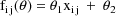
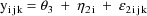
The statistical model for the jth observation from the ith individual is taken to be

where and are regression parameters, denotes weight, the are statistically independent values of random interindividual effects, with means 0 and common variance (a scalar), and the are statistically independent values of random intraindividual effects, with means 0 and common variance (a scalar). A value of the random interindividual effect, , is always taken to be statistically independent of a value of the random intraindividual effect, . The variable x is doubly subscripted, suggesting that for each individual, its value can vary between doses. In fact, though, in the actual data set its value remains constant across doses for each individual. The regression function is linear in weight. Since if this linearity holds, it may do so only over a limited weight range, an intercept parameter might be included in the model. However, analysis of the data has revealed no evidence whatsoever of a nonzero intercept. Consequently, while an intercept parameter has in fact been included in the model, in this example it shall be constrained to be 0. Under the model, the observations , , ..., are each affected by , and so they are correlated. 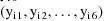We let denote the column form of the vector consisting of the six observations, . The random intraindividual effect is clearly nested within the random interindividual effect. For each value of the random interindividual effect, the random intraindividual effect takes on six different values, while for no value of the random intraindividual effect does the random interindividual effect take on different values. (These effects are presumed to be continuously distributed.)

The NONMEM linear model schematic is given by

where

Let I denote the number of individuals. Also, for fixed i, let denote the column vector of values of the , let denote the column vector of values of the (viz. a column vector of 1’s), and let denote the column vector of values of the (viz. a column vector of 1’s). Then the ELS objective function is given by

where

and where if A is a square matrix, denotes the diagonal matrix whose diagonal elements are those of A. The matrix is the variance-covariance matrix of . The vector is the vector of weighted residuals from the observations . As with previous examples, it has the form residual (vector) divided by standard deviation (matrix), and it is "squared" in the expression for the objective function. The weighted residuals are defined to be the weighted residuals from all obervations . It may be seen that the form of the objective function is the same as that given with previous examples, except that now has an extra term expressing intraindividual variability which for the first time is a factor.

E.3. Implementation of Example 1 E.3.1. Inputs

A code for PRED which implements the example is given in Fig. 57. Note that the values and are returned in G(1) and H(1), respectively. These are the coefficients of and in the NONMEM linear model schematic. In general, the value returned in G(I) is the coefficient of the Ith random interindividual effect in the NONMEM linear model schematic, and the value returned returned in H(I) is the coefficient of the Ith random intraindividual effect in the NONMEM linear model schematic.

A control stream for this example is given in Fig. 58. The data set is embedded in it, and the data items in a data record are the ID, weight, and DV data items, respectively.

Since in the example there are both random inter- and intra-individual effects, there are entries in both fields 2 and 3 of the initial STRUCTURE record. In general, the numbers of random interindividual effects and random intraindividual effects are placed in fields 2 and 3, respectively. The total number of both random inter- and intra-individual effects cannot exceed 10. Also, since in the example both and are taken to be diagonal (they are both scalars), there are 1’s in both fields 6 and 8. In general, if is constrained to be diagonal, a 1 is placed in field 6, and if is constrained to be diagonal, a 1 is placed in field 8. If ( ) is not constrained, a 1 is placed in field 7 (9). (Since a scalar is also an unconstrained matrix, in this example a 1 could be placed in either field 7 or 9, but a more perspicuous problem summary develops when a scalar is regarded as a diagonal matrix.)

The initial estimate of is obtained by first averaging all the 72 clearances to obtain an estimate of mean clearance in the population. (This is equivalent to averaging the 6 clearances in each of the 12 individuals to obtain to obtain estimates of the individuals’ mean clearances, and then averaging these 12 individual estimates.) Then this estimate is divided by 70Kg, the average weight of the individuals of the sample, to obtain the desired estimate. Since lower and upper bounds of 0 are specified for (thus this parameter is fixed to 0), lower and upper bounds must also be specified for , but these are taken to be and (see sections C.3.4.4 and C.3.4.5).

Since in the example the two parameters and must be estimated, as well as , there must be initial estimates specified for each. Therefore, a DIAGONAL record for , as well as a DIAGONAL record for appears in the problem specification. Its form is exactly that of the DIAGONAL record for . The initial estimate record for (be it a DIAGONAL or BLOCK SET record) is placed after the initial estimate record for (be it a DIAGONAL or BLOCK SET record).

Unlike previous examples, for illustrative purposes, actual initial estimates have been placed in both DIAGONAL records, rather than letting the fields be blank. The initial estimate of is obtained by first obtaining for each individual, the sample variance of his clearance measurements. Then these individual estimates are averaged to obtain the desired estimate. The initial estimate of is obtained by first calculating the sample variance of the individuals’ average clearances. Then 1/6 of the the initial estimate of is subtracted from this sample variance to obtain the desired estimate. In this example the same final estimate, standard errors, etc. are obtained when the fields of the DIAGONAL records are left blank.

E.3.2 Selected Printout

The final parameter estimate, standard errors, and correlation matrix are shown in Figs. 59-61. Note that in these printouts is listed. Its final estimate is 0, the value to which the parameter is fixed. The covariance (or correlation) of any estimate of a fixed parameter with the estimate of any other parameter is by definition 0. However, lest the user forget this and think that a number other than 0 could appear for the estimate of this covariance (or correlation), but that 0 is in fact the estimate, a 0 does not in fact appear in the printout. Instead, a place holder consisting of dots appears in order to remind the user that the covariance (correlation) is 0 by definition. Similarly, this type of place holder also appears for the standard error estimate of the point estimate of a fixed parameter.

The two scatterplots of residual vs weight and weighted residual vs weight are shown in Figs. 62 and 63. It is not necessary to separate these scatterplots by ID since in this example weight is in effect a surrogate for ID, and so the residuals are already very naturally separated by individual. However, to better look for homogeneous scatter, it is better to examine the scatterplot of weighted residual vs weight. In this example the weighted residuals are distributed much more homogeneously about the zero line than are the residuals.

E.4. Example with Two Inter- and Two Intra-individual Random Effects

This is an extension of example 1. Again, six oral doses are given to each of 12 subjects, and with each dose a clearance is measured. In addition, with each dose a rate constant of elimination is measured. This measurement is an estimate of the parameter in the example of section D.4, obtained graphically from the plasma concentration vs time data ocurring after the absorption phase is over. The clearance and rate constant may correlate across doses within any individual. Therefore, the clearance and rate constant together form a bivariate observation from the point of view of random intraindividual variablity. There are altogether 6 such bivariate observations per individual.

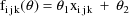
The statistical model for the kth element of the jth (bivariate) observation from the ith individual is taken to be

where is a clearance-rate constant indicator variable (0: clearance; 1: rate constant). Here the new part of the model is the part for the rate constant measurement. The mean rate constant measurement is simply assumed to be a constant and not to vary with weight. The error structure for the rate constant measurements is analogous to that for the clearance mesurements; it is the sum of both simple interindividual and simple intraindividual error. The variance-covariance matrix of is the matrix , and the variance-covariance matrix of is the matrix . A value of the random interindividual effect vector is always statistically independent of a value of the random intraindividual effect vector . Under the model the clearance observations from individual i are each affected by the , the rate constant observations from individual i are each affected by , and and are correlated, and so all the observations from individual i are correlated. Each pair of clearance and rate constant observations with a given dose are also correlated by virtue of the correlation between the two random intraindividual effects. We let denote the column form of the vector consisting of the twelve observations, . The random intraindividual effects are clearly nested within the random interindividual effects.

The NONMEM linear model schematic is given by

where

Let I denote the number of individuals. Also, for fixed i, let denote the column vector of values of the , let denote the column vector of values of the , let denote the column vector of values of the , let denote the column vector of values of the , and let denote the column vector of values of the . Then the ELS objective function is given by

where

and where if A is a square matrix, denotes the block diagonal matrix whose diagonal blocks are the diagonal blocks of A. The matrix is the variance-covariance matrix of . The vector is the vector of weighted residuals from the observations . As with previous examples, it has the form residual (vector) divided by standard deviation (matrix), and it is "squared" in the expression for the objective function. The weighted residuals are defined to be the weighted residuals from all obervations .

E.5 Implementation of Example 2

E.5.1 Inputs

A code for PRED which implements the example is given in Fig. 64. The computation involves querying the value of . Note that the values and are returned in G(1) and G(2), respectively. These are the coefficients of and in the NONMEM linear model schematic. In general, the value returned in G(I) is the coefficient of the Ith random interindividual effect in the NONMEM linear model schematic. The values and are returned in H(1) and H(2), respectively. These are the coefficients of and in the NONMEM linear model schematic. In general, the value returned in H(I) is the coefficient of the Ith random intraindividual effect in the NONMEM linear model schematic.

A control stream for this example is given in Fig. 65. The data set is embedded in it, and the data items in a data record are the ID data item, the weight data item, the DV data item, the clearance-rate constant indicator data item ( ), and the level-two data item, respectively. This last type of data item is needed with one-level nested random effects in order to group together the DV data items belonging to a bivariate observation (see section B.1). It is given the label L2 in the NONMEM printout, and the ID data item is given the label L1 since in this example the ID data item is also the level-one data item. Note that for readability and for the purpose of conveniently keying the data, the indicator data item is blank in those places where it is actually zero, and similarly with the level-two data item. The alternating use of the values 0 and 1 for the level-two data items illustrates how it is not necessary that noncontiguous level-two records have different level-two data items. Note that the index of the level-two data item is placed in field 7 of the ITEM record.

The initial STRUCTURE record for the problem specification has 1’s in fields 7 and 9, indicating that both and are full matrices, i.e. neither is constrained to be diagonal. When a 1 is placed in field 7 (9) of the initial STRUCTURE record, the number of random inter- (intra-) individual effects cannot exceed 5.

The control stream contains a STRUCTURE record for , as well as a STRUCTURE record for . This is, of course, because neither nor is constrained to be a diagonal matrix. The form of the STRUCTURE record for is exactly that of the STRUCTURE record for (see section D.5.2). When the STRUCTURE record for appears, it is placed after the STRUCTURE record for , except when the latter record is not present, in which case the STRUCTURE record for is placed after the initial STRUCTURE record.

The initial estimate for is that used in the previous example. The initial estimate of is obtained by averaging the 72 rate constant measurements.

The control stream contains a BLOCK SET record for , as well as a BLOCK SET record for . The form of the BLOCK SET record for is exactly that of the BLOCK SET record for (see section D.5.3).

The initial estimate of is obtained by first obtaining for each individual, the sample variance-covariance matrix of his clearance and rate constant measurements. Then these individual matrix estimates are averaged to obtain the desired estimate. The initial estimate of is obtained by first calculating the sample variance-covariance matrix of the individuals’ average clearances and average rate constants. Then 1/6 of the the initial estimate of is subtracted from this sample variance-covariance matrix to obtain the desired estimate. In this example the same final estimate, standard errors, etc. are obtained when the fields of the BLOCK SET records are left blank.

E.5.2 Selected Printout

The final estimate, standard errors, and correlation matrix are shown in Figs. 66-68. It is interesting to compare the final estimates and standard errors from this example with those from the previous example. All the parameters associated with clearance only that occur in the model with the previous example also occur in the extension of that model which is considered here, and in this extended model the only parameter associated with both clearance and rate constant is the covariance parameter in . Consequently, the final estimates and standard errors of the estimates from this example are very close to those from the previous example.

Regarding the covariance parameter , note that its normalized value, i.e. the correlation between and ( ), is estimated to be .95. (Whereas the minimum value of the objective function is -651, in another NONMEM run where is constrained to be DIAGONAL the minimum value is much larger -631, indicating that the correlation is indeed significant.) This suggests that variablity in estimates of volume of distribution that might be obtained across individuals and doses would be due largely to random intraindividual (dose to dose) variablity and little to random interindividual variablity. The reason for this is as follows. As noted in section E.2, a clearance observation for a given individual and dose might have been measured by , where and are estimates of the rate constant of elimination and volume of distribution obtained from concentration vs time data. As noted in section E.4, a rate constant observation for a given individual and dose might have been measured by . The high interindividual correlation between these two types of measurements implies an approximately proportional interindividual relationship between and , i.e. an approximately constant interindividual relationship for .

The first and last pages of the requested table are shown in Fig. 69. The scatterplots of residual vs weight separated by TYPE are given Figs. 70 and 71. The scatterplots of weighted residual vs weight separated by TYPE are given in Figs. 72 and 73.

TOP

TABLE OF CONTENTS

NEXT